【时间序列预测】基于matlab RBF神经网络时间序列预测【含Matlab源码 1336期】

一、RBF神经网络简介
1 RBF网络
径向基函数(RBF)网络是一种向前网络,它以函数逼近理论为基础,能够逼近任意非线性的函数,同时具有很好的泛化能力和较快的学习速度。RBF神经网络由输入层、隐含层、输出层组成。输入层由输入节点组成,只传递输入信号到隐含层;隐含层由神经元的变换函数,如高斯函数、格林函数等辐射状作用函数构成,其中隐含层节点数由问题的实际需求来确定;输出层是对输入的响应,由输入节点组成。
RBF网络的主要思想是:将输入数据直接映射到隐含层空间,用径向基函数作为隐单元的“基”构成隐含层的空间,在此空间对输入数据进行变换,将在低维空间中的非线性数据变换为高维空间内线性可分。这种非线性的映射关系,通过径向基函数的中心点来确定。输出层则是通过隐含层的线性映射得到的,即网络的输出是隐含层神经单元输出的线性加权和。具体结构如图1所示。
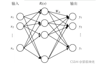
图1 RBF神经网络结构
隐含层节点中的作用函数(基函数)对输入信号将在局部产生响应。最常用的基函数是高斯函数,如下:

式中:x是n维输入向量;ci是第i个基函数的中心,与x具有相同维数的向量;σi是第i个感知的变量,决定基函数中心点的宽度;m是感知单元的个数;

令输入层实现从x→Ri(x)的非线性映射,隐含层实现从Ri(x)到yk的线性映射,即:

式中:r是输出节点数;wik是权值。
由上述RBF网络的原理可知,RBF网络主要涉及三种可调参数:RBF的中心向量ci、偏值σi、隐含层到输出层的权重wik。其中,RBF的中心ci的选取对网络性能至关重要,中心太近,会产生近似线性相关;中心太远,产生的网络会过大。根据这三种参数的确定,可以将RBF网络划分为很多种学习方法,最常见的是:随机选取中心法、自组织选取中心法、有监督选取中心法和正交最小二乘法(OLS)。
2 时间序列的RBF神经网络预测
基于RBF神经网络的时间序列预测模型,最主要的是需要确定好训练样本的输入和输出。为预测时间序列y(i)的值,以X(i)=[y(i-n),y(i-n+1),…,y(i-1)]T作为输入,n为历史数据长度,代表过去n天的历史数据。因此网络结构[11]可以表示为y(i)=f(y(in),y(i-n+1),…,y(i-1))。
由于时间序列有一定的复杂性,而且序列数据前后的关联程度大不相同。因此,采用不同的历史数据长度的预测模型,结果大相径庭。本文分别采用不同的历史数据长度,选取其中预测结果均方误差最小的历史数据长度,提高模型的预测性能。
二、部分源代码
%% Mackey Glass Time Series Prediction using Spatio-Temporal Radial Basis Function (RBF) Neural Network
% Author: Shujaat Khan, shujaat123@gmail.com
clc;
clear all;
close all;
%% Loading Time Series Data
% I generated a series x(t) for t = 0,1, . . . ,3000, using mackey glass series equation with the following configurations: b = 0.1, a = 0.2, Tau = 20, and the initial conditions x(t - Tau) = 0.
load Dataset/Data.mat
% Training and Test datasets
time_steps=2; % prediction of #time_steps forward value (for this simple architechture time_steps<=3)
% Training
start_of_series_tr=100;
end_of_series_tr=2500;
% Test
start_of_series_ts=2500;
end_of_series_ts=3000;
P_train=Data(start_of_series_tr:end_of_series_tr-time_steps,2); % Input Data
f_train=Data(start_of_series_tr+time_steps:end_of_series_tr,2); % Label Data (desired output values)
indt=Data(start_of_series_tr+time_steps:end_of_series_tr,1);% Time index
SNR = 30; % signal to noise ratio
f_train=awgn(f_train,SNR); % Adding white Gaussian noise
%% Simulation parameters
% Defining architechture of the RBF-NN
[m n] = size(P_train);% Dimensions of input data [m]-length of signal, [n]-number of elements in each input
order=2; % Number of past values used for the prediction of future value
n1 = 10; % Number of hidden layer neurons
% Tuning parameters for training
epoch=10; % simulation rounds (number of times the same data pass through the NN for training)
eta=5e-2; % Gradient Descent step-size (learning rate)
runs=10; % Number of Monte Carlo simulations
Iti=[]; % Initial mean square error (MSE)
% Graphics/Plot parameters
fsize=13; % Fontsize
lw=2; % line width size
%% Training Phase
for run=1:runs % Monte Carlos simulations loop
% spread and centers of the Gaussian kernel
[temp, c, beeta] = kmeans(P_train,n1); % K-means clustering
% c=[c awgn(c,10)];
beeta=2*beeta; % Increasing spread of Gaussian kernel
% Initialization of weights and bias
w=randn(order,n1); % weight
b=randn(); % bias
for k=1:epoch % simulation rounds loop
I(k)=0; % reset MSE
U=zeros(1,order); % reset input vector
for i1=1:m % Iteration loop
% sliding window (updating input vector)
U(1:end-1)=U(2:end);
U(end)=P_train(i1); % current value of time-series
% Gaussian Kernel
for i2=1:n1
phi(:,i2)=exp((-(abs(U-c(i2,:))))/beeta(i2,:).^2);
end
% Calculate output of the RBF
y_train(i1)=sum(sum(w.*phi))+b;
e(i1)=f_train(i1)-y_train(i1); % instantaneous error in the prediction
% Gradient descent-based weight-update rule
w=w+eta*e(i1)*phi;
b=b+eta*e(i1);
% Mean square error
I(i1)=mse(e(1:i1)); % Objective Function
end
Itti(epoch,:)=I; % MSE for all iterations
end
Iti(run,:)=mean(Itti,1); % Mean MSE for all epochs
end
It=mean(Iti,1); % Mean MSE for all independent runs (Monte Carlo simulations)
%% Test Phase
P_test=Data(start_of_series_ts:end_of_series_ts-time_steps,2);
f_test=Data(start_of_series_ts+time_steps:end_of_series_ts,2);
indts=Data(start_of_series_ts+time_steps:end_of_series_ts,1);
[m n] = size(P_test);
for i1=1:m % Iteration loop
% sliding window (updating input vector)
U(1:end-1)=U(2:end);
U(end)=P_test(i1);
for i2=1:n1
phi(:,i2)=exp((-(abs(U-c(i2,:))))/beeta(i2,:).^2);
end
y_test(i1)=sum(sum(w.*phi))+b;
e_test(i1)=real(f_test(i1)-y_test(i1));
I(2400+i1)=mse(e_test(1:i1));
end
save ST_RBF.mat
% %% Results
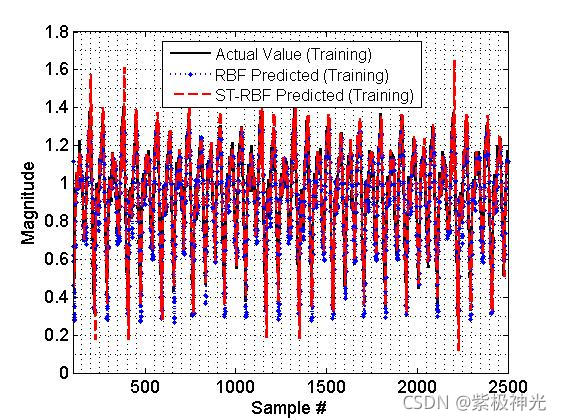
% % Input and output signals (training phase)
% figure
% plot(indt,f_train,'k','linewidth',lw);
% hold on;
% plot(indt,y_train,'.:b','linewidth',lw);
% xlim([start_of_series_tr+time_steps end_of_series_tr]);
% h=legend('Actual Value (Training)','RBF Predicted (Training)','Location','Best');
% grid minor
% xlabel('Sample #','FontSize',fsize);
% ylabel('Magnitude','FontSize',fsize);
% set(h,'FontSize',12)
% set(gca,'FontSize',13)
% saveas(gcf,strcat('Time_SeriesTraining.png'),'png')
%
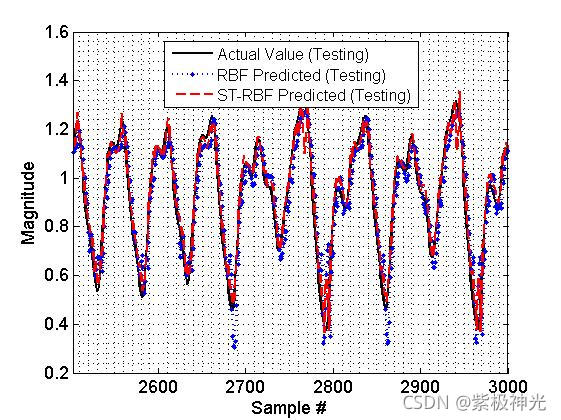
% % Input and output signals (test phase)
% figure
% plot(indts,f_test,'k','linewidth',lw);
% hold on;
% plot(indts,y_test,'.:b','linewidth',lw);
% xlim([start_of_series_ts+time_steps end_of_series_ts]);
% h=legend('Actual Value (Testing)','RBF Predicted (Testing)','Location','Best');
% grid minor
% xlabel('Sample #','FontSize',fsize);
% ylabel('Magnitude','FontSize',fsize);
% set(h,'FontSize',12)
% set(gca,'FontSize',13)
% saveas(gcf,strcat('Time_SeriesTesting.png'),'png')
%
% % Objective function (MSE) (training phase)
% figure
% plot(start_of_series_tr:end_of_series_tr-1,10*log10(I(1:end_of_series_tr-start_of_series_tr)),'+-b','linewidth',lw)
% h=legend('RBF (Training)','Location','North');
% grid minor
% xlabel('Sample #','FontSize',fsize);
% ylabel('MSE (dB)','FontSize',fsize);
% set(h,'FontSize',12)
% set(gca,'FontSize',13)
% saveas(gcf,strcat('Time_SeriesTrainingMSE.png'),'png')
%
% % Objective function (MSE) (test phase)
% figure
% plot(start_of_series_ts+time_steps:end_of_series_ts,10*log10(I(end_of_series_tr-start_of_series_tr+1:end)),'.:b','linewidth',lw+1)
% h=legend('RBF (Testing)','Location','South');
% grid minor
% xlabel('Sample #','FontSize',fsize);
% ylabel('MSE (dB)','FontSize',fsize);
% set(h,'FontSize',12)
% set(gca,'FontSize',13)
% saveas(gcf,strcat('Time_SeriesTestingMSE.png'),'png')
%
% % Mean square error
% 10*log10(((f_train'-y_train)*(f_train'-y_train)')/length(y_train))
% 10*log10(((f_test'-y_test)*(f_test'-y_test)')/length(y_test))
Results_graphs
- 1
- 2
- 3
- 4
- 5
- 6
- 7
- 8
- 9
- 10
- 11
- 12
- 13
- 14
- 15
- 16
- 17
- 18
- 19
- 20
- 21
- 22
- 23
- 24
- 25
- 26
- 27
- 28
- 29
- 30
- 31
- 32
- 33
- 34
- 35
- 36
- 37
- 38
- 39
- 40
- 41
- 42
- 43
- 44
- 45
- 46
- 47
- 48
- 49
- 50
- 51
- 52
- 53
- 54
- 55
- 56
- 57
- 58
- 59
- 60
- 61
- 62
- 63
- 64
- 65
- 66
- 67
- 68
- 69
- 70
- 71
- 72
- 73
- 74
- 75
- 76
- 77
- 78
- 79
- 80
- 81
- 82
- 83
- 84
- 85
- 86
- 87
- 88
- 89
- 90
- 91
- 92
- 93
- 94
- 95
- 96
- 97
- 98
- 99
- 100
- 101
- 102
- 103
- 104
- 105
- 106
- 107
- 108
- 109
- 110
- 111
- 112
- 113
- 114
- 115
- 116
- 117
- 118
- 119
- 120
- 121
- 122
- 123
- 124
- 125
- 126
- 127
- 128
- 129
- 130
- 131
- 132
- 133
- 134
- 135
- 136
- 137
- 138
- 139
- 140
- 141
- 142
- 143
- 144
- 145
- 146
- 147
- 148
- 149
- 150
- 151
- 152
- 153
- 154
- 155
- 156
- 157
- 158
- 159
- 160
- 161
- 162
- 163
- 164
- 165
- 166
- 167
三、运行结果
四、matlab版本及参考文献
1 matlab版本
2014a
2 参考文献
[1] 包子阳,余继周,杨杉.智能优化算法及其MATLAB实例(第2版)[M].电子工业出版社,2016.
[2]张岩,吴水根.MATLAB优化算法源代码[M].清华大学出版社,2017.
[3]周品.MATLAB 神经网络设计与应用[M].清华大学出版社,2013.
[4]陈明.MATLAB神经网络原理与实例精解[M].清华大学出版社,2013.
[5]方清城.MATLAB R2016a神经网络设计与应用28个案例分析[M].清华大学出版社,2018.
[6]黄伟建,张丽娜,黄远,程瑶.RBF神经网络在河流营养盐预测中的应用[J].现代电子技术. 2019,42(20)
文章来源: qq912100926.blog.csdn.net,作者:海神之光,版权归原作者所有,如需转载,请联系作者。
原文链接:qq912100926.blog.csdn.net/article/details/120472670

- 点赞
- 收藏
- 关注作者
评论(0)