@[toc]

摘要

本例提取了植物幼苗数据集中的部分数据做数据集，数据集共有12种类别，今天我和大家一起实现tensorflow2.X版本图像分类任务，分类的模型使用EfficientNetB0。

通过这篇文章你可以学到：

1、如何加载图片数据，并处理数据。

2、如果将标签转为onehot编码

3、如何使用数据增强。

4、如何使用mixup。

5、如何切分数据集。

6、如何加载预训练模型。

EfficientNet简介

EfficientNet是谷歌2019年提出的分类模型，自从提出以后这个模型，各大竞赛平台常常能看到他的身影，成了霸榜的神器。下图是EfficientNet—B0模型的网络结构。

从网络中可以看出，作者构建了MBConv，结构如下图：

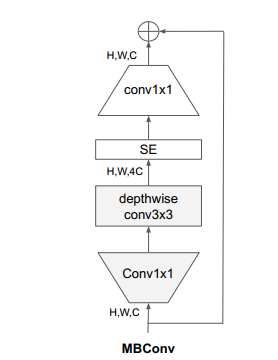
k对应的卷积核的大小，经过1×1的卷积，然后channel放大4倍，再经过depthwise conv3×3的卷积，然后经过SE模块后，再经过1×1的卷积，把channel恢复到输入的大小，最后和上层的输入融合。

项目结构

EfficientNet_demo
├─data
│  ├─test
│  └─train
│      ├─Black-grass
│      ├─Charlock
│      ├─Cleavers
│      ├─Common Chickweed
│      ├─Common wheat
│      ├─Fat Hen
│      ├─Loose Silky-bent
│      ├─Maize
│      ├─Scentless Mayweed
│      ├─Shepherds Purse
│      ├─Small-flowered Cranesbill
│      └─Sugar beet
├─mixupgenerator.py
├─train.py
├─test1.py
└─test.py

训练

1、Mixup

mixup是一种非常规的数据增强方法，一个和数据无关的简单数据增强原则，其以线性插值的方式来构建新的训练样本和标签。最终对标签的处理如下公式所示，这很简单但对于增强策略来说又很不一般。

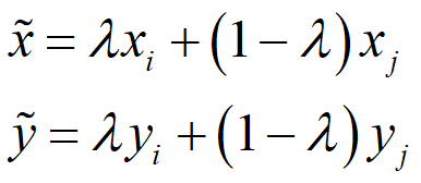
$\left ( x_{i},y_{i} \right )$, $\left ( x_{j},y_{j} \right )$两个数据对是原始数据集中的训练样本对（训练样本和其对应的标签）。其中 $\lambda$是一个服从B分布的参数, $\lambda\sim Beta\left ( \alpha ,\alpha \right )$ 。Beta分布的概率密度函数如下图所示，其中 $\alpha \in \left [ 0,+\infty \right ]$

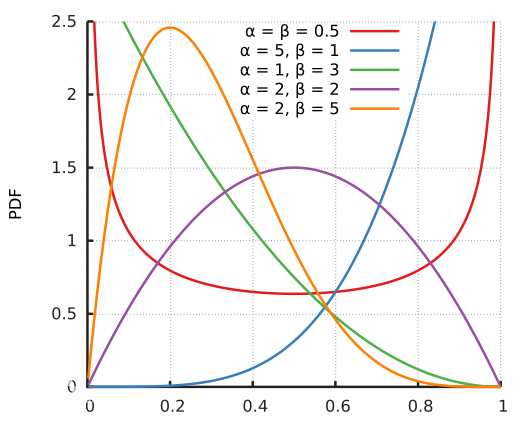
因此 $\alpha$是一个超参数，随着 $\alpha$的增大，网络的训练误差就会增加，而其泛化能力会随之增强。而当 $\alpha \rightarrow \infty$时，模型就会退化成最原始的训练策略。参考：https://www.jianshu.com/p/d22fcd86f36d

新建mixupgenerator.py，插入一下代码：

import numpy as np


class MixupGenerator():
    def __init__(self, X_train, y_train, batch_size=32, alpha=0.2, shuffle=True, datagen=None):
        self.X_train = X_train
        self.y_train = y_train
        self.batch_size = batch_size
        self.alpha = alpha
        self.shuffle = shuffle
        self.sample_num = len(X_train)
        self.datagen = datagen

    def __call__(self):
        while True:
            indexes = self.__get_exploration_order()
            itr_num = int(len(indexes) // (self.batch_size * 2))

            for i in range(itr_num):
                batch_ids = indexes[i * self.batch_size * 2:(i + 1) * self.batch_size * 2]
                X, y = self.__data_generation(batch_ids)

                yield X, y

    def __get_exploration_order(self):
        indexes = np.arange(self.sample_num)

        if self.shuffle:
            np.random.shuffle(indexes)

        return indexes

    def __data_generation(self, batch_ids):
        _, h, w, c = self.X_train.shape
        l = np.random.beta(self.alpha, self.alpha, self.batch_size)
        X_l = l.reshape(self.batch_size, 1, 1, 1)
        y_l = l.reshape(self.batch_size, 1)

        X1 = self.X_train[batch_ids[:self.batch_size]]
        X2 = self.X_train[batch_ids[self.batch_size:]]
        X = X1 * X_l + X2 * (1 - X_l)

        if self.datagen:
            for i in range(self.batch_size):
                X[i] = self.datagen.random_transform(X[i])
                X[i] = self.datagen.standardize(X[i])

        if isinstance(self.y_train, list):
            y = []

            for y_train_ in self.y_train:
                y1 = y_train_[batch_ids[:self.batch_size]]
                y2 = y_train_[batch_ids[self.batch_size:]]
                y.append(y1 * y_l + y2 * (1 - y_l))
        else:
            y1 = self.y_train[batch_ids[:self.batch_size]]
            y2 = self.y_train[batch_ids[self.batch_size:]]
            y = y1 * y_l + y2 * (1 - y_l)

        return X, y

2、 导入需要的数据包，设置全局参数

import os
import pickle
import cv2
import numpy as np
from sklearn.metrics import classification_report
from sklearn.model_selection import train_test_split
from sklearn.preprocessing import LabelBinarizer
from tensorflow.keras.applications import EfficientNetB0
from tensorflow.keras.optimizers import Adam
from tensorflow.keras.preprocessing.image import img_to_array
from tensorflow.python.keras.callbacks import ModelCheckpoint, ReduceLROnPlateau
from tensorflow.python.keras.layers import Dense
from tensorflow.python.keras.models import Sequential

from mixupgenerator import MixupGenerator

norm_size = 224
datapath = 'data/train'
EPOCHS = 100
INIT_LR = 3e-4
labelList = []
classnum = 12
batch_size = 16

这里可以看出tensorflow2.0以上的版本集成了Keras，我们在使用的时候就不必单独安装Keras了，以前的代码升级到tensorflow2.0以上的版本将keras前面加上tensorflow即可。

tensorflow说完了，再说明一下几个重要的全局参数：

• norm_size = 224 ，EfficientNetB0默认的图片尺寸是224×224。

• datapath = ‘data/train’, 设置图片存放的路径，在这里要说明一下如果图片很多，一定不要放在工程目录下，否则Pycharm加载工程的时候会浏览所有的图片，很慢很慢。

• EPOCHS = 300, epochs的数量，关于epoch的设置多少合适，这个问题很纠结，一般情况设置300足够了，如果感觉没有训练好，再载入模型训练。

• INIT_LR = 3e-4,学习率，一般情况从0.001开始逐渐降低，也别太小了到1e-6就可以了。

• classnum = 12, 类别数量，数据集有12个类别，所有就定义12类。

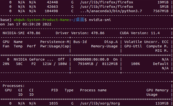
• batch_size = 16，batchsize，根据硬件的情况和数据集的大小设置，太小了loss浮动太大，太大了收敛不好，根据经验来，一般设置为2的次方。windows可以通过任务管理器查看显存的占用情况。

  

  Ubuntu可以使用nvidia-smi查看显存的占用。

  

3、 加载图片

处理图像的步骤:

1. 读取图像
2. 用指定的大小去resize图像。
3. 将图像转为数组
4. 图像归一化
5. 使用LabelBinarizer将标签转为onehot编码.

具体做法详见代码：

def loadImageData():
    imageList = []
    listClasses = os.listdir(datapath)# 类别文件夹
    for class_name in listClasses:
        class_path=os.path.join(datapath,class_name)
        image_names=os.listdir(class_path)
        for image_name in image_names:
            image_full_path = os.path.join(class_path, image_name)
            labelList.append(class_name)
            image = cv2.imdecode(np.fromfile(image_full_path, dtype=np.uint8), -1)
            image = cv2.resize(image, (norm_size, norm_size), interpolation=cv2.INTER_LANCZOS4)
            if image.shape[2] >3:
                image=image[:,:,:3]
                print(image.shape)
            image = img_to_array(image)
            imageList.append(image)
    imageList = np.array(imageList) / 255.0
    return imageList


print("开始加载数据")
imageArr = loadImageData()
print("加载数据完成")
print(labelList)
lb = LabelBinarizer()
labelList = lb.fit_transform(labelList)
print(labelList)
print(lb.classes_)
f = open('label_bin.pickle', "wb")
f.write(pickle.dumps(lb))
f.close()

做好数据之后，我们需要切分训练集和测试集，一般按照4：1或者7：3的比例来切分。切分数据集使用train_test_split()方法，需要导入from sklearn.model_selection import train_test_split 包。例：

trainX, valX, trainY, valY = train_test_split(imageArr, labelList, test_size=0.2, random_state=42)

4、图像增强

ImageDataGenerator()是keras.preprocessing.image模块中的图片生成器，同时也可以在batch中对数据进行增强，扩充数据集大小，增强模型的泛化能力。比如进行旋转，变形，归一化等等。

keras.preprocessing.image.ImageDataGenerator(featurewise_center=False,samplewise_center
=False, featurewise_std_normalization=False, samplewise_std_normalization=False,zca_whitening=False,
 zca_epsilon=1e-06, rotation_range=0.0, width_shift_range=0.0, height_shift_range=0.0,brightness_range=None, shear_range=0.0, zoom_range=0.0,channel_shift_range=0.0, fill_mode='nearest', cval=0.0, horizontal_flip=False, vertical_flip=False, rescale=None, preprocessing_function=None,data_format=None,validation_split=0.0)

参数:

• featurewise_center: Boolean. 对输入的图片每个通道减去每个通道对应均值。
• samplewise_center: Boolan. 每张图片减去样本均值, 使得每个样本均值为0。
• featurewise_std_normalization(): Boolean()
• samplewise_std_normalization(): Boolean()
• zca_epsilon(): Default 12-6
• zca_whitening: Boolean. 去除样本之间的相关性
• rotation_range(): 旋转范围
• width_shift_range(): 水平平移范围
• height_shift_range(): 垂直平移范围
• shear_range(): float, 透视变换的范围
• zoom_range(): 缩放范围
• fill_mode: 填充模式, constant, nearest, reflect
• cval: fill_mode == 'constant’的时候填充值
• horizontal_flip(): 水平反转
• vertical_flip(): 垂直翻转
• preprocessing_function(): user提供的处理函数
• data_format(): channels_first或者channels_last
• validation_split(): 多少数据用于验证集

本例使用的图像增强代码如下：

from tensorflow.keras.preprocessing.image import ImageDataGenerator

train_datagen = ImageDataGenerator(
                                   rotation_range=20,
                                   width_shift_range=0.2,
                                   height_shift_range=0.2,
                                   horizontal_flip=True)
val_datagen = ImageDataGenerator()  # 验证集不做图片增强
training_generator_mix = MixupGenerator(trainX, trainY, batch_size=batch_size, alpha=0.2, datagen=train_datagen)()
val_generator = val_datagen.flow(valX, valY, batch_size=batch_size, shuffle=True)

注意：只在训练集上做增强，不在验证集上做增强。

5、 保留最好的模型和动态设置学习率

ModelCheckpoint：用来保存成绩最好的模型。

语法如下：

keras.callbacks.ModelCheckpoint(filepath, monitor='val_loss', verbose=0, save_best_only=False, save_weights_only=False, mode='auto', period=1)

该回调函数将在每个epoch后保存模型到filepath

filepath可以是格式化的字符串，里面的占位符将会被epoch值和传入on_epoch_end的logs关键字所填入

例如，filepath若为weights.{epoch:02d-{val_loss:.2f}}.hdf5，则会生成对应epoch和验证集loss的多个文件。

参数

• filename：字符串，保存模型的路径
• monitor：需要监视的值
• verbose：信息展示模式，0或1
• save_best_only：当设置为True时，将只保存在验证集上性能最好的模型
• mode：‘auto’，‘min’，‘max’之一，在save_best_only=True时决定性能最佳模型的评判准则，例如，当监测值为val_acc时，模式应为max，当检测值为val_loss时，模式应为min。在auto模式下，评价准则由被监测值的名字自动推断。
• save_weights_only：若设置为True，则只保存模型权重，否则将保存整个模型（包括模型结构，配置信息等）
• period：CheckPoint之间的间隔的epoch数

ReduceLROnPlateau：当评价指标不在提升时，减少学习率，语法如下：

keras.callbacks.ReduceLROnPlateau(monitor='val_loss', factor=0.1, patience=10, verbose=0, mode='auto', epsilon=0.0001, cooldown=0, min_lr=0)

当学习停滞时，减少2倍或10倍的学习率常常能获得较好的效果。该回调函数检测指标的情况，如果在patience个epoch中看不到模型性能提升，则减少学习率

参数

• monitor：被监测的量
• factor：每次减少学习率的因子，学习率将以lr = lr*factor的形式被减少
• patience：当patience个epoch过去而模型性能不提升时，学习率减少的动作会被触发
• mode：‘auto’，‘min’，‘max’之一，在min模式下，如果检测值触发学习率减少。在max模式下，当检测值不再上升则触发学习率减少。
• epsilon：阈值，用来确定是否进入检测值的“平原区”
• cooldown：学习率减少后，会经过cooldown个epoch才重新进行正常操作
• min_lr:学习率的下限

本例代码如下：

checkpointer = ModelCheckpoint(filepath='best_model.hdf5',
                               monitor='val_accuracy', verbose=1, save_best_only=True, mode='max')

reduce = ReduceLROnPlateau(monitor='val_accuracy', patience=10,
                           verbose=1,
                           factor=0.5,
                           min_lr=1e-6)

6、建立模型并训练

model = Sequential()
model.add(EfficientNetB0(input_shape=(224, 224, 3), include_top=False, pooling='avg', weights='imagenet'))
model.add(Dense(classnum, activation='softmax'))
model.summary()
optimizer = Adam(learning_rate=INIT_LR)
model.compile(optimizer=optimizer, loss='categorical_crossentropy', metrics=['accuracy'])

history = model.fit(training_generator_mix,
                    steps_per_epoch=trainX.shape[0] / batch_size,
                    validation_data=val_generator,
                    epochs=EPOCHS,
                    validation_steps=valX.shape[0] / batch_size,
                    callbacks=[checkpointer, reduce])
model.save('my_model.h5')

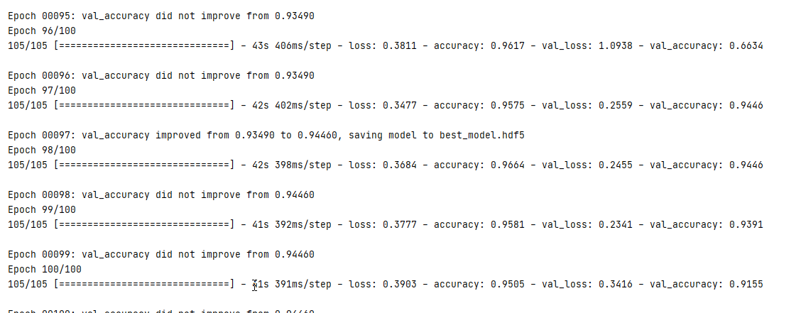
运行结果：

训练了100个epoch，准确率已经过达到了0.94。

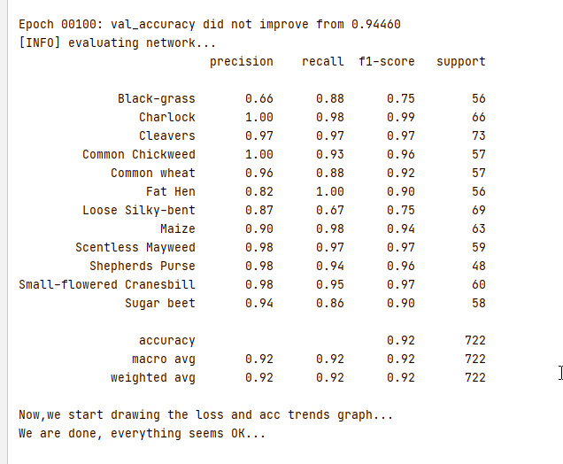
7、模型评估

使用classification_report对验证集做评估，导入包from sklearn.metrics import classification_report

predictions = model.predict(x=valX, batch_size=16)
print(classification_report(valY.argmax(axis=1),
	predictions.argmax(axis=1), target_names=lb.classes_))

运行结果如下：

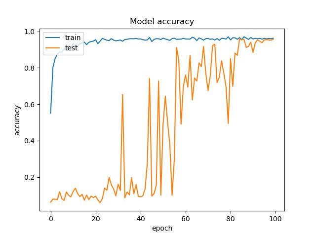
8、保留训练结果，并将其生成图片

loss_trend_graph_path = r"WW_loss.jpg"
acc_trend_graph_path = r"WW_acc.jpg"
import matplotlib.pyplot as plt

print("Now,we start drawing the loss and acc trends graph...")
# summarize history for accuracy
fig = plt.figure(1)
plt.plot(history.history["accuracy"])
plt.plot(history.history["val_accuracy"])
plt.title("Model accuracy")
plt.ylabel("accuracy")
plt.xlabel("epoch")
plt.legend(["train", "test"], loc="upper left")
plt.savefig(acc_trend_graph_path)
plt.close(1)
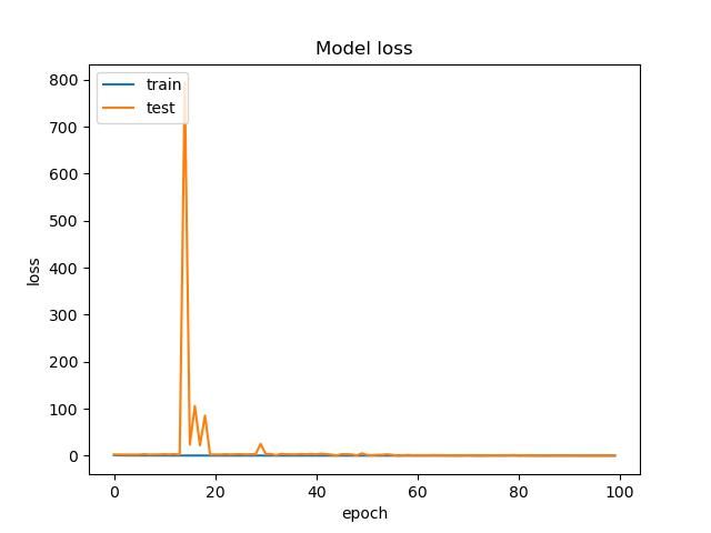
# summarize history for loss
fig = plt.figure(2)
plt.plot(history.history["loss"])
plt.plot(history.history["val_loss"])
plt.title("Model loss")
plt.ylabel("loss")
plt.xlabel("epoch")
plt.legend(["train", "test"], loc="upper left")
plt.savefig(loss_trend_graph_path)
plt.close(2)
print("We are done, everything seems OK...")
# #windows系统设置10关机
#os.system("shutdown -s -t 10")

结果：

测试部分

单张图片预测

1、导入依赖

import pickle
import cv2
import numpy as np
from tensorflow.keras.preprocessing.image import img_to_array
from  tensorflow.keras.models import load_model
import time

2、设置全局参数

这里注意，字典的顺序和训练时的顺序保持一致

norm_size=224
imagelist=[]
emotion_labels = {
    0: 'Black-grass',
    1: 'Charlock',
    2: 'Cleavers',
    3: 'Common Chickweed',
    4: 'Common wheat',
    5: 'Fat Hen',
    6: 'Loose Silky-bent',
    7: 'Maize',
    8: 'Scentless Mayweed',
    9: 'Shepherds Purse',
    10: 'Small-flowered Cranesbill',
    11: 'Sugar beet',
}

3、加载模型

这里要加载两个模型，一个是LabelBinarizer模型，一个是MobileNetV3Large模型。

emotion_classifier=load_model("best_model.hdf5")
lb = pickle.loads(open("label_bin.pickle", "rb").read())
t1=time.time()

4、处理图片

处理图片的逻辑和训练集也类似，步骤：

• 读取图片
• 将图片resize为norm_size×norm_size大小。
• 将图片转为数组。
• 放到imagelist中。
• imagelist整体除以255，把数值缩放到0到1之间。

image = cv2.imdecode(np.fromfile('data/test/0a64e3e6c.png', dtype=np.uint8), -1)
# load the image, pre-process it, and store it in the data list
image = cv2.resize(image, (norm_size, norm_size), interpolation=cv2.INTER_LANCZOS4)
image = img_to_array(image)
imagelist.append(image)
imageList = np.array(imagelist, dtype="float") / 255.0

5、预测类别

预测类别，并获取最高类别的index。

out=emotion_classifier.predict(imageList)
print(out)
pre=np.argmax(out)
label = lb.classes_[pre]
t2=time.time()
print(label)
t3=t2-t1
print(t3)

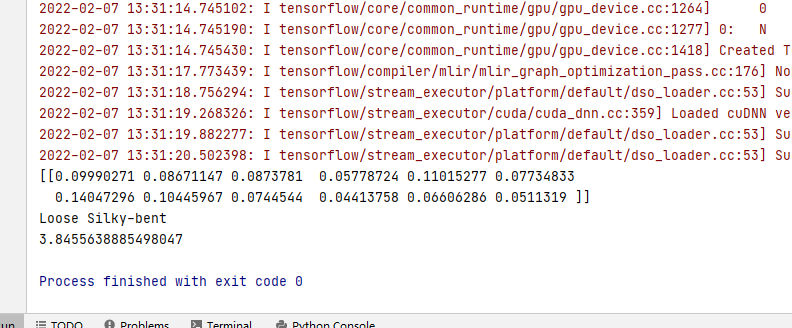
运行结果：

批量预测

批量预测和单张预测的差别主要在读取数据上，以及预测完成后，对预测类别的处理。其他的没有变化。

步骤：

• 加载模型。
• 定义测试集的目录
• 获取目录下的图片
• 循环循环图片
  • 读取图片
  • resize图片
  • 转数组
  • 放到imageList中
• 缩放到0到255.
• 预测

emotion_classifier=load_model("best_model.hdf5")
lb = pickle.loads(open("label_bin.pickle", "rb").read())
t1=time.time()
predict_dir = 'data/test'
test11 = os.listdir(predict_dir)
for file in test11:
    filepath=os.path.join(predict_dir,file)

    image = cv2.imdecode(np.fromfile(filepath, dtype=np.uint8), -1)
    # load the image, pre-process it, and store it in the data list
    image = cv2.resize(image, (norm_size, norm_size), interpolation=cv2.INTER_LANCZOS4)
    image = img_to_array(image)
    imagelist.append(image)
imageList = np.array(imagelist, dtype="float") / 255.0
out = emotion_classifier.predict(imageList)
print(out)
pre = [np.argmax(i) for i in out]
class_name_list=[lb.classes_[i] for i in pre]
print(class_name_list)
t2 = time.time()
t3 = t2 - t1
print(t3)

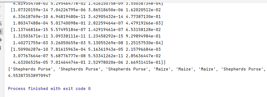
运行结果：

完整代码：
https://download.csdn.net/download/hhhhhhhhhhwwwwwwwwww/79581688