【RNN入门到实战】LSTM从入门到实战——实现空气质量预测

摘要
LSTM是一种时间递归神经网络,它出现的原因是为了解决RNN的一个致命的缺陷。RNN在处理长期依赖(时间序列上距离较远的节点)时,因为计算距离较远的节点之间的联系时会涉及雅可比矩阵的多次相乘,会造成梯度消失或者梯度膨胀的现象。为了解决该问题,研究人员提出了许多解决办法,例如ESN(Echo State Network),增加有漏单元(Leaky Units)等等。其中最成功应用最广泛的就是门限RNN(Gated RNN),而LSTM就是门限RNN中最著名的一种。有漏单元通过设计连接间的权重系数,从而允许RNN累积距离较远节点间的长期联系;而门限RNN则泛化了这样的思想,允许在不同时刻改变该系数,且允许网络忘记当前已经累积的信息。

RNN和LSTM的区别
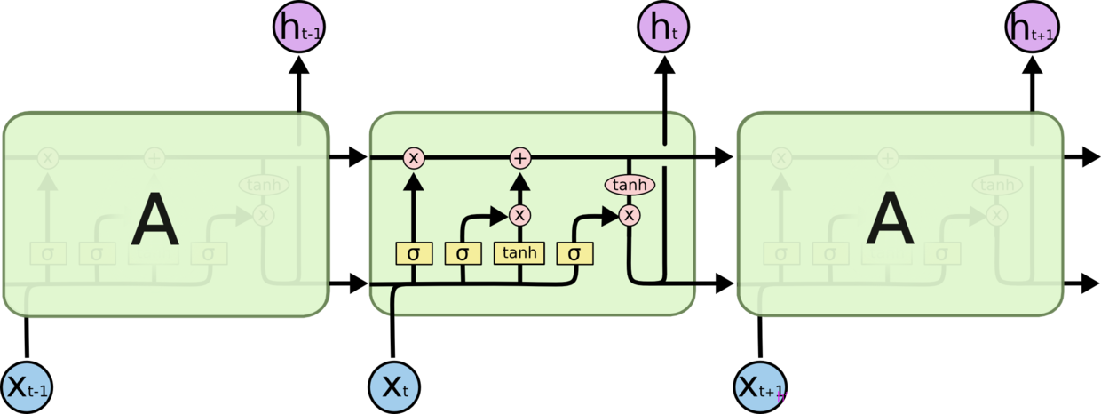
所有 RNN 都具有一种重复神经网络模块的链式的形式。在标准的 RNN 中,这个重复的模块只有一个非常简单的结构,例如一个 tanh 层,如下图所示:
 LSTM 同样是这样的结构,但是重复的模块拥有一个不同的结构。不同于单一神经网络层,这里是有四个,以一种非常特殊的方式进行交互。
详解LSTM
LSTM 的关键就是Cell状态,水平线在图上方贯穿运行。Cell状态类似于传送带。直接在整个链上运行,只有一些少量的线性交互。信息在上面流传保持不变会很容易。示意图如下所示:

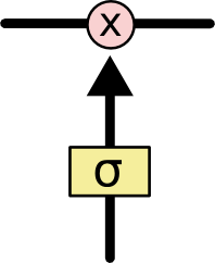
LSTM 有通过精心设计的称作为“门”的结构来去除或者增加信息到Cell状态的能力。门是一种让信息选择式通过的方法。他们包含一个 sigmoid 神经网络层和一个 pointwise 乘法操作。示意图如下:
忘记层门
h t − 1 h_{t-1} ht−1 x t x_t xt C t − 1 C_{t-1} Ct−1

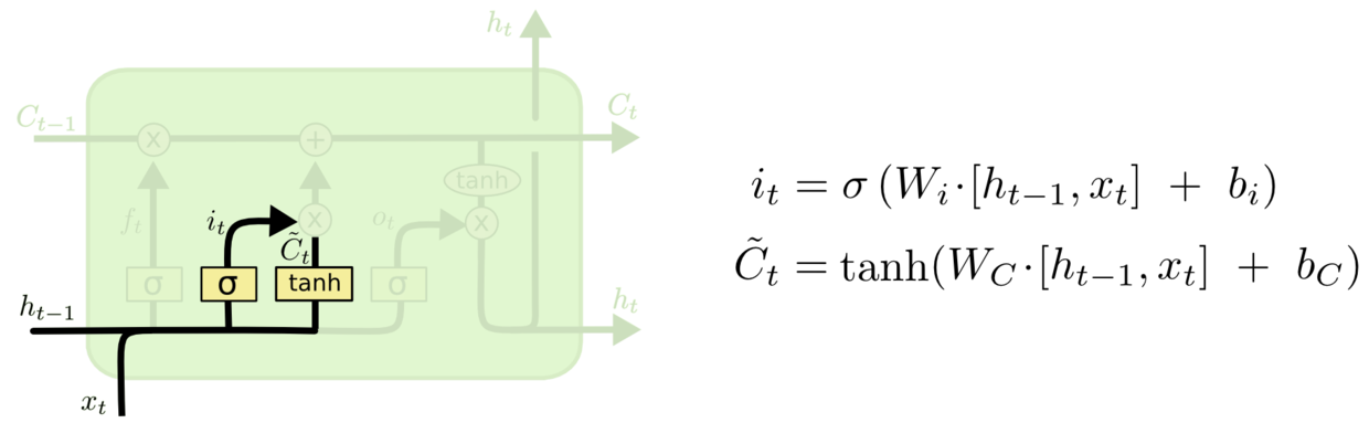
输入层门
作用对象:细胞状态
作用:将新的信息选择性的记录到细胞状态中。
操作步骤:
步骤一,sigmoid 层称 “输入门层” 决定什么值我们将要更新。
步骤二,tanh 层创建一个新的候选值向量 C ~ t \tilde{C}_t C~t加入到状态中。其示意图如下:
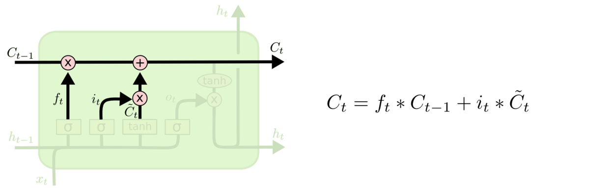
步骤三:将 c t − 1 c_{t-1} ct−1更新为 c t c_{t} ct。将旧状态与 f t f_t ft相乘,丢弃掉我们确定需要丢弃的信息。接着加上 i t ∗ C ~ t i_t * \tilde{C}_t it∗C~t得到新的候选值,根据我们决定更新每个状态的程度进行变化。其示意图如下:
动图演示

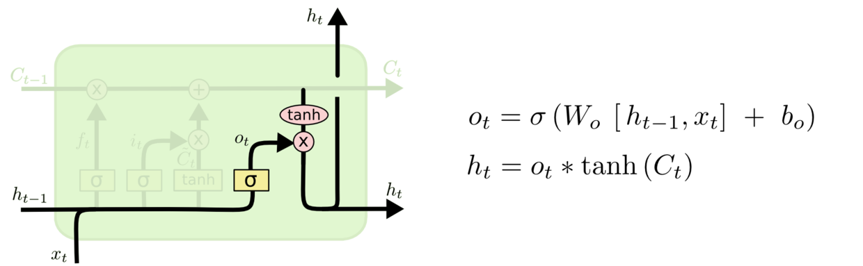
输出层门
作用对象:隐层 h t h_t ht
作用:确定输出什么值。
操作步骤:
步骤一:通过sigmoid 层来确定细胞状态的哪个部分将输出。
步骤二:把细胞状态通过 tanh 进行处理,并将它和 sigmoid 门的输出相乘,最终我们仅仅会输出我们确定输出的那部分。
其示意图如下所示:
动图演示

实战——使用LSTM实现空气质量预测
数据来源自位于北京的美国大使馆在2010年至2014年共5年间每小时采集的天气及空气污染指数。
数据集包括日期、PM2.5浓度、露点、温度、风向、风速、累积小时雪量和累积小时雨量。原始数据中完整的特征如下:
1.No 行数
2.year 年
3.month 月
4.day 日
5.hour 小时
6.pm2.5 PM2.5浓度
7.DEWP 露点
8.TEMP 温度
9.PRES 大气压
10.cbwd 风向
11.lws 风速
12.ls 累积雪量
13.lr 累积雨量
我们可以利用此数据集搭建预测模型,利用前一个或几个小时的天气条件和污染数据预测下一个(当前)时刻的污染程度。
数据处理
首先,我们必须清洗数据。以下是原始数据集的前几行。
No  year  month  day  hour  pm2.5  DEWP  TEMP    PRES cbwd    Iws  Is  Ir
0   1  2010      1    1     0    NaN   -21 -11.0  1021.0   NW   1.79   0   0
1   2  2010      1    1     1    NaN   -21 -12.0  1020.0   NW   4.92   0   0
2   3  2010      1    1     2    NaN   -21 -11.0  1019.0   NW   6.71   0   0
3   4  2010      1    1     3    NaN   -21 -14.0  1019.0   NW   9.84   0   0
4   5  2010      1    1     4    NaN   -20 -12.0  1018.0   NW  12.97   0   0
5   6  2010      1    1     5    NaN   -19 -10.0  1017.0   NW  16.10   0   0
6   7  2010      1    1     6    NaN   -19  -9.0  1017.0   NW  19.23   0   0
7   8  2010      1    1     7    NaN   -19  -9.0  1017.0   NW  21.02   0   0
8   9  2010      1    1     8    NaN   -19  -9.0  1017.0   NW  24.15   0   0
9  10  2010      1    1     9    NaN   -20  -8.0  1017.0   NW  27.28   0   0
- 1
- 2
- 3
- 4
- 5
- 6
- 7
- 8
- 9
- 10
- 11
数据理清的步骤:
1、将year, month, day, hour四列整合为一个日期时间。
2、删除No列,这个列对于数据预测没有作用,如果有作用说明见鬼了。
3、将数据集中所有的NaN设置为0,NaN没有办法用来计算。
4、删除前24行,前24行的pm2.5没有记录,留着没有用。
完整的代码如下:
from pandas import read_csv
from datetime import datetime
# load data
def parse(x):
    return datetime.strptime(x, '%Y %m %d %H')
# 读取数据,将year, month, day, hour四列合并成一列。
dataset = read_csv('raw.csv',  parse_dates = [['year', 'month', 'day', 'hour']], index_col=0, date_parser=parse)
# 删除No列
dataset.drop('No', axis=1, inplace=True)
# 修改列名
dataset.columns = ['pollution', 'dew', 'temp', 'press', 'wnd_dir', 'wnd_spd', 'snow', 'rain']
dataset.index.name = 'date'
print(dataset)
# 将所有的NaN设置为0
dataset['pollution'].fillna(0, inplace=True)
# 删除前24行
dataset = dataset[24:]
# 浏览前5行数据
print(dataset.head(5))
# save to file
dataset.to_csv('pollution.csv')
- 1
- 2
- 3
- 4
- 5
- 6
- 7
- 8
- 9
- 10
- 11
- 12
- 13
- 14
- 15
- 16
- 17
- 18
- 19
- 20
- 21
- 22
加载了“pollution.csv”文件,并对除了类别型特性“风速”的每一列数据分别绘图。
  dataset = pd.read_csv('pollution.csv', header=0, index_col=0)
    values = dataset.values
    # specify columns to plot
    groups = [0, 1, 2, 3, 5, 6, 7]
    i = 1
    # plot each column
    pyplot.figure(figsize=(10, 10))
    for group in groups:
        pyplot.subplot(len(groups), 1, i)
        pyplot.plot(values[:, group])
        pyplot.title(dataset.columns[group], y=0.5, loc='right')
        i += 1
    pyplot.show()
- 1
- 2
- 3
- 4
- 5
- 6
- 7
- 8
- 9
- 10
- 11
- 12
- 13
运行上面的代码,并对7个变量在5年的范围内绘图。 
利用sklearn的预处理模块对类别特征“风向”进行编码,当然也可以对该特征进行one-hot编码。 接着对所有的特征进行归一化处理,然后将数据集转化为有监督学习问题,同时将需要预测的当前时刻(t)的天气条件特征移除,代码如下:
def series_to_supervised(data, n_in=1, n_out=1, dropnan=True):
    # convert series to supervised learning
    n_vars = 1 if type(data) is list else data.shape[1]
    df = pd.DataFrame(data)
    cols, names = list(), list()
    # input sequence (t-n, ... t-1)
    for i in range(n_in, 0, -1):
        cols.append(df.shift(i))
        names += [('var%d(t-%d)' % (j + 1, i)) for j in range(n_vars)]
    # forecast sequence (t, t+1, ... t+n)
    for i in range(0, n_out):
        cols.append(df.shift(-i))
        if i == 0:
            names += [('var%d(t)' % (j + 1)) for j in range(n_vars)]
        else:
            names += [('var%d(t+%d)' % (j + 1, i)) for j in range(n_vars)]
    # put it all together
    agg = pd.concat(cols, axis=1)
    agg.columns = names
    # drop rows with NaN values
    if dropnan:
        agg.dropna(inplace=True)
    return agg
# load dataset
dataset = pd.read_csv('pollution.csv', header=0, index_col=0)
values = dataset.values
# integer encode direction
encoder = LabelEncoder()
print(values[:, 4])
values[:, 4] = encoder.fit_transform(values[:, 4])
print(values[:, 4])
# ensure all data is float
values = values.astype('float32')
# normalize features
scaler = MinMaxScaler(feature_range=(0, 1))
scaled = scaler.fit_transform(values)
# frame as supervised learning
reframed = series_to_supervised(scaled, 1, 1)
# drop columns we don't want to predict
reframed.drop(reframed.columns[[9, 10, 11, 12, 13, 14, 15]], axis=1, inplace=True)
print(reframed.head())
- 1
- 2
- 3
- 4
- 5
- 6
- 7
- 8
- 9
- 10
- 11
- 12
- 13
- 14
- 15
- 16
- 17
- 18
- 19
- 20
- 21
- 22
- 23
- 24
- 25
- 26
- 27
- 28
- 29
- 30
- 31
- 32
- 33
- 34
- 35
- 36
- 37
- 38
- 39
- 40
- 41
构造模型
首先,我们需要将处理后的数据集划分为训练集和测试集。为了加速模型的训练,我们仅利用第一年数据进行训练,然后利用剩下的4年进行评估。
下面的代码将数据集进行划分,然后将训练集和测试集划分为输入和输出变量,最终将输入(X)改造为LSTM的输入格式,即[samples,timesteps,features]。
# split into train and test sets
values = reframed.values
n_train_hours = 365 * 24
train = values[:n_train_hours, :]
test = values[n_train_hours:, :]
# split into input and outputs
train_X, train_y = train[:, :-1], train[:, -1]
test_X, test_y = test[:, :-1], test[:, -1]
# reshape input to be 3D [samples, timesteps, features]
train_X = train_X.reshape((train_X.shape[0], 1, train_X.shape[1]))
test_X = test_X.reshape((test_X.shape[0], 1, test_X.shape[1]))
print(train_X.shape, train_y.shape, test_X.shape, test_y.shape)
- 1
- 2
- 3
- 4
- 5
- 6
- 7
- 8
- 9
- 10
- 11
- 12
运行上述代码打印训练集和测试集的输入输出格式,其中9K小时数据作训练集,35K小时数据作测试集。
(8760, 1, 8) (8760,) (35039, 1, 8) (35039,)
现在可以搭建LSTM模型了。 LSTM模型中,隐藏层有50个神经元,输出层1个神经元(回归问题),输入变量是一个时间步(t-1)的特征,损失函数采用Mean Absolute Error(MAE),优化算法采用Adam,模型采用50个epochs并且每个batch的大小为72。
最后,在fit()函数中设置validation_data参数,记录训练集和测试集的损失,并在完成训练和测试后绘制损失图。
checkpointer = ModelCheckpoint(filepath='best_model.hdf5', monitor='val_loss', verbose=1, save_best_only=True,
                                   mode='min')
reduce = ReduceLROnPlateau(monitor='val_loss', patience=10, verbose=1, factor=0.5, min_lr=1e-6)

model = Sequential()
model.add(LSTM(50, input_shape=(train_X.shape[1], train_X.shape[2])))
model.add(Dense(1))
model.compile(loss='mae', optimizer='adam')
    # fit network
history = model.fit(train_X, train_y, epochs=300, batch_size=64, validation_data=(test_X, test_y), verbose=1,
                        callbacks=[checkpointer, reduce],
                        shuffle=True)
    # plot history
pyplot.plot(history.history['loss'], label='train')
pyplot.plot(history.history['val_loss'], label='test')
pyplot.legend()
pyplot.show()
- 1
- 2
- 3
- 4
- 5
- 6
- 7
- 8
- 9
- 10
- 11
- 12
- 13
- 14
- 15
- 16
- 17
模型评估
接下里我们对模型效果进行评估。
值得注意的是:需要将预测结果和部分测试集数据组合然后进行比例反转(invert the scaling),同时也需要将测试集上的预期值也进行比例转换。
(We combine the forecast with the test dataset and invert the scaling. We also invert scaling on the test dataset with the expected pollution numbers.)
至于在这里为什么进行比例反转,是因为我们将原始数据进行了预处理(连同输出值y),此时的误差损失计算是在处理之后的数据上进行的,为了计算在原始比例上的误差需要将数据进行转化。同时笔者有个小Tips:就是反转时的矩阵大小一定要和原来的大小(shape)完全相同,否则就会报错。
通过以上处理之后,再结合RMSE(均方根误差)计算损失。
yhat = model.predict(test_X)
test_X = test_X.reshape((test_X.shape[0], test_X.shape[2]))
# invert scaling for forecast
inv_yhat = concatenate((yhat, test_X[:, 1:]), axis=1)
inv_yhat = scaler.inverse_transform(inv_yhat)
inv_yhat = inv_yhat[:, 0]
# invert scaling for actual
inv_y = scaler.inverse_transform(test_X)
inv_y = inv_y[:, 0]
# calculate RMSE
rmse = sqrt(mean_squared_error(inv_y, inv_yhat))
print('Test RMSE: %.3f' % rmse)
- 1
- 2
- 3
- 4
- 5
- 6
- 7
- 8
- 9
- 10
- 11
- 12
完整代码
import pandas as pd
from datetime import datetime
from matplotlib import pyplot
from sklearn.preprocessing import LabelEncoder, MinMaxScaler
from sklearn.metrics import mean_squared_error
from tensorflow.keras.models import Sequential
from tensorflow.keras.layers import Dense
from tensorflow.keras.layers import LSTM
from numpy import concatenate
from math import sqrt


# load data
def parse(x):
    return datetime.strptime(x, '%Y %m %d %H')


def read_raw():
    dataset = pd.read_csv('raw.csv', parse_dates=[['year', 'month', 'day', 'hour']], index_col=0, date_parser=parse)
    dataset.drop('No', axis=1, inplace=True)
    # manually specify column names
    dataset.columns = ['pollution', 'dew', 'temp', 'press', 'wnd_dir', 'wnd_spd', 'snow', 'rain']
    dataset.index.name = 'date'
    # mark all NA values with 0
    dataset['pollution'].fillna(0, inplace=True)
    # drop the first 24 hours
    dataset = dataset[24:]
    # summarize first 5 rows
    print(dataset.head(5))
    # save to file
    dataset.to_csv('pollution.csv')


def drow_pollution():
    dataset = pd.read_csv('pollution.csv', header=0, index_col=0)
    values = dataset.values
    # specify columns to plot
    groups = [0, 1, 2, 3, 5, 6, 7]
    i = 1
    # plot each column
    pyplot.figure(figsize=(10, 10))
    for group in groups:
        pyplot.subplot(len(groups), 1, i)
        pyplot.plot(values[:, group])
        pyplot.title(dataset.columns[group], y=0.5, loc='right')
        i += 1
    pyplot.show()


def series_to_supervised(data, n_in=1, n_out=1, dropnan=True):
    # convert series to supervised learning
    n_vars = 1 if type(data) is list else data.shape[1]
    df = pd.DataFrame(data)
    cols, names = list(), list()
    # input sequence (t-n, ... t-1)
    for i in range(n_in, 0, -1):
        cols.append(df.shift(i))
        names += [('var%d(t-%d)' % (j + 1, i)) for j in range(n_vars)]
    # forecast sequence (t, t+1, ... t+n)
    for i in range(0, n_out):
        cols.append(df.shift(-i))
        if i == 0:
            names += [('var%d(t)' % (j + 1)) for j in range(n_vars)]
        else:
            names += [('var%d(t+%d)' % (j + 1, i)) for j in range(n_vars)]
    # put it all together
    agg = pd.concat(cols, axis=1)
    agg.columns = names
    # drop rows with NaN values
    if dropnan:
        agg.dropna(inplace=True)
    return agg


def cs_to_sl():
    # load dataset
    dataset = pd.read_csv('pollution.csv', header=0, index_col=0)
    values = dataset.values
    # integer encode direction
    encoder = LabelEncoder()
    print(values[:, 4])
    values[:, 4] = encoder.fit_transform(values[:, 4])
    print(values[:, 4])
    # ensure all data is float
    values = values.astype('float32')
    # normalize features
    scaler = MinMaxScaler(feature_range=(0, 1))
    scaled = scaler.fit_transform(values)
    # frame as supervised learning
    reframed = series_to_supervised(scaled, 1, 1)
    # drop columns we don't want to predict
    reframed.drop(reframed.columns[[9, 10, 11, 12, 13, 14, 15]], axis=1, inplace=True)
    print(reframed.head())
    return reframed, scaler


def train_test(reframed):
    # split into train and test sets
    values = reframed.values
    n_train_hours = 365 * 24
    train = values[:n_train_hours, :]
    test = values[n_train_hours:, :]
    # split into input and outputs
    train_X, train_y = train[:, :-1], train[:, -1]
    test_X, test_y = test[:, :-1], test[:, -1]
    # reshape input to be 3D [samples, timesteps, features]
    train_X = train_X.reshape((train_X.shape[0], 1, train_X.shape[1]))
    test_X = test_X.reshape((test_X.shape[0], 1, test_X.shape[1]))
    print(train_X.shape, train_y.shape, test_X.shape, test_y.shape)
    return train_X, train_y, test_X, test_y


def fit_network(train_X, train_y, test_X, test_y, scaler):
    print(train_X.shape)
    print(train_X.shape[1])
    model = Sequential()
    model.add(LSTM(50, input_shape=(train_X.shape[1], train_X.shape[2])))
    model.add(Dense(1))
    model.compile(loss='mae', optimizer='adam')
    # fit network
    history = model.fit(train_X, train_y, epochs=50, batch_size=72, validation_data=(test_X, test_y), verbose=2,
                        shuffle=False)
    # plot history
    pyplot.plot(history.history['loss'], label='train')
    pyplot.plot(history.history['val_loss'], label='test')
    pyplot.legend()
    pyplot.show()
    # make a prediction
    yhat = model.predict(test_X)
    test_X = test_X.reshape((test_X.shape[0], test_X.shape[2]))
    # invert scaling for forecast
    inv_yhat = concatenate((yhat, test_X[:, 1:]), axis=1)
    inv_yhat = scaler.inverse_transform(inv_yhat)
    inv_yhat = inv_yhat[:, 0]
    # invert scaling for actual
    inv_y = scaler.inverse_transform(test_X)
    inv_y = inv_y[:, 0]
    # calculate RMSE
    rmse = sqrt(mean_squared_error(inv_y, inv_yhat))
    print('Test RMSE: %.3f' % rmse)


if __name__ == '__main__':
    drow_pollution()
    reframed, scaler = cs_to_sl()
    train_X, train_y, test_X, test_y = train_test(reframed)
    fit_network(train_X, train_y, test_X, test_y, scaler)
- 1
- 2
- 3
- 4
- 5
- 6
- 7
- 8
- 9
- 10
- 11
- 12
- 13
- 14
- 15
- 16
- 17
- 18
- 19
- 20
- 21
- 22
- 23
- 24
- 25
- 26
- 27
- 28
- 29
- 30
- 31
- 32
- 33
- 34
- 35
- 36
- 37
- 38
- 39
- 40
- 41
- 42
- 43
- 44
- 45
- 46
- 47
- 48
- 49
- 50
- 51
- 52
- 53
- 54
- 55
- 56
- 57
- 58
- 59
- 60
- 61
- 62
- 63
- 64
- 65
- 66
- 67
- 68
- 69
- 70
- 71
- 72
- 73
- 74
- 75
- 76
- 77
- 78
- 79
- 80
- 81
- 82
- 83
- 84
- 85
- 86
- 87
- 88
- 89
- 90
- 91
- 92
- 93
- 94
- 95
- 96
- 97
- 98
- 99
- 100
- 101
- 102
- 103
- 104
- 105
- 106
- 107
- 108
- 109
- 110
- 111
- 112
- 113
- 114
- 115
- 116
- 117
- 118
- 119
- 120
- 121
- 122
- 123
- 124
- 125
- 126
- 127
- 128
- 129
- 130
- 131
- 132
- 133
- 134
- 135
- 136
- 137
- 138
- 139
- 140
- 141
- 142
- 143
- 144
- 145
- 146
- 147
代码和数据集链接:https://download.csdn.net/download/hhhhhhhhhhwwwwwwwwww/19781047
文章来源: wanghao.blog.csdn.net,作者:AI浩,版权归原作者所有,如需转载,请联系作者。
原文链接:wanghao.blog.csdn.net/article/details/118088119

- 点赞
- 收藏
- 关注作者
评论(0)