多标签分类算法详解及实践(Keras)

目录
多标签分类
multi-label classification problem:多标签分类(或者叫多标记分类),是指一个样本的标签数量不止一个,即一个样本对应多个标签。
如何使用多标签分类
在预测多标签分类问题时,假设隐藏层的输出是[-1.0, 5.0, -0.5, 5.0, -0.5 ],如果用softmax函数的话,那么输出为:
z = np.array([-1.0, 5.0, -0.5, 5.0, -0.5])print(Softmax_sim(z))# 输出为[ 0.00123281 0.49735104 0.00203256 0.49735104 0.00203256]
通过使用softmax,我们可以清楚地选择标签2和标签4。但我们必须知道每个样本需要多少个标签,或者为概率选择一个阈值。这显然不是我们想要的,因为样本属于每个标签的概率应该是独立的。
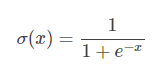
对于一个二分类问题,常用的激活函数是sigmoid函数:
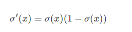
ps: sigmoid函数之所以在之前很长一段时间作为神经网络激活函数(现在大家基本都用Relu了),一个很重要的原因是sigmoid函数的导数很容易计算,可以用自身表示:
python 代码为:
-
import numpy as np
-
-
def Sigmoid_sim(x):
-
return 1 /(1+np.exp(-x))
-
-
a = np.array([-1.0, 5.0, -0.5, 5.0, -0.5])
-
print(Sigmoid_sim(a))
-
#输出为: [ 0.26894142 0.99330715 0.37754067 0.99330715 0.37754067]
此时,每个标签的概率即是独立的。完整整个模型构建之后,最后一步中最重要的是为模型的编译选择损失函数。在多标签分类中,大多使用binary_crossentropy损失而不是通常在多类分类中使用的categorical_crossentropy损失函数。这可能看起来不合理,但因为每个输出节点都是独立的,选择二元损失,并将网络输出建模为每个标签独立的bernoulli分布。整个多标签分类的模型为:
-
from keras.models import Model
-
from keras.layers import Input,Dense
-
-
inputs = Input(shape=(10,))
-
hidden = Dense(units=10,activation='relu')(inputs)
-
output = Dense(units=5,activation='sigmoid')(hidden)
-
model.compile(optimizer='adam', loss='binary_crossentropy', metrics=['accuracy'])
多标签使用实例
我们使用最常用的衣服数据集来实现多标签分类,网络模型使用ResNet50。
数据集地址:链接:https://pan.baidu.com/s/1eANXTnWl2nf853IEiLOvWg
提取码:jo4h
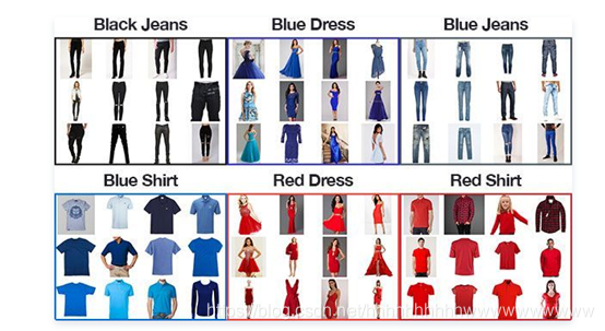
我们的数据集由5547张图片组成,它们来自12个不同的种类,包括:
- black_dress(333张图片)
- black_jeans(344张图片)
- black_shirt(436张图片)
- black_shoe(534张图片)
- blue_dress(386张图片)
- blue_jeans(356张图片)
- blue_shirt(369张图片)
- red_dress(384张图片)
- red_shirt(332张图片)
- red_shoe(486张图片)
- white_bag(747张图片)
- white_shoe(840张图片)
我们的卷积神经网络的目标是同时预测颜色和服饰类别。代码使用Tensorflow2.0以上版本编写。下面对我实现算法的代码作讲解:
训练
引入库,设置超参数
-
# import the necessary packages
-
-
from sklearn.preprocessing import MultiLabelBinarizer
-
from sklearn.model_selection import train_test_split
-
from imutils import paths
-
import tensorflow as tf
-
import numpy as np
-
import argparse
-
import random
-
import pickle
-
import cv2
-
import os
-
from tensorflow.python.keras.applications.resnet import ResNet50
-
from tensorflow.keras.optimizers import Adam
-
from tensorflow.python.keras.callbacks import ModelCheckpoint, ReduceLROnPlateau
-
from tensorflow.python.keras.preprocessing.image import ImageDataGenerator, img_to_array
-
-
# construct the argument parse and parse the arguments
-
-
ap = argparse.ArgumentParser()
-
ap.add_argument("-d", "--dataset", default='../dataset',
-
help="path to input dataset (i.e., directory of images)")
-
ap.add_argument("-m", "--model", default='model.h5',
-
help="path to output model")
-
ap.add_argument("-l", "--labelbin", default='labelbin',
-
help="path to output label binarizer")
-
ap.add_argument("-p", "--plot", type=str, default="plot.png",
-
help="path to output accuracy/loss plot")
-
args = vars(ap.parse_args())
超参数的解释:
- --dataset:输入的数据集路径。
- --model:输出的Keras序列模型路径。
- --labelbin:输出的多标签二值化对象路径。
- --plot:输出的训练损失及正确率图像路径。
设置全局参数
-
EPOCHS = 150
-
-
INIT_LR = 1e-3
-
-
BS = 16
-
-
IMAGE_DIMS = (224, 224, 3)
加载数据
print("[INFO] loading images...")
imagePaths = sorted(list(paths.list_images(args["dataset"])))
random.seed(42)
random.shuffle(imagePaths)
# initialize the data and labels
data = []
labels = []
# loop over the input images
for imagePath in imagePaths:
# load the image, pre-process it, and store it in the data list
image = cv2.imread(imagePath)
image = cv2.resize(image, (IMAGE_DIMS[1], IMAGE_DIMS[0]))
image = img_to_array(image)
data.append(image)
# extract set of class labels from the image path and update the
# labels list
l = label = imagePath.split(os.path.sep)[-2].split("_")
labels.append(l)
# scale the raw pixel intensities to the range [0, 1]
data = np.array(data, dtype="float") / 255.0
labels = np.array(labels)
print(labels)
运行结果:
[['red' 'shirt']
['black' 'jeans']
['black' 'shoe']
...
['black' 'dress']
['black' 'shirt']
['white' 'shoe']]
生成多分类的标签
print("[INFO] class labels:")
mlb = MultiLabelBinarizer()
labels = mlb.fit_transform(labels)
# loop over each of the possible class labels and show them
for (i, label) in enumerate(mlb.classes_):
print("{}. {}".format(i + 1, label))
print(labels)
通过MultiLabelBinarizer()的fit就可以得到label的编码。我们将类别和生成后的标签打印出来。类别结果如下:
[INFO] class labels:
1. bag
2. black
3. blue
4. dress
5. jeans
6. red
7. shirt
8. shoe
9. white
lables的输出结果如下:
[[0 0 0 ... 1 0 0]
[0 1 0 ... 0 0 0]
[0 1 0 ... 0 1 0]
...
[0 1 0 ... 0 0 0]
[0 1 0 ... 1 0 0]
[0 0 0 ... 0 1 1]]
为了方便大家理解标签,我通过下面的表格说明
|
|
Bag |
Black |
Blue |
Dress |
Jeans |
Red |
Shirt |
Shoe |
White |
| [‘red’ ’shirt’] |
0 |
0 |
0 |
0 |
0 |
1 |
1 |
0 |
0 |
| [‘black’ ’jeans’] |
0 |
1 |
0 |
0 |
1 |
0 |
0 |
0 |
0 |
| ['white' 'shoe'] |
0 |
0 |
0 |
0 |
0 |
0 |
0 |
1 |
1 |
然后,将MultiLabelBinarizer()训练的模型保存,方便测试时使用。代码如下:
print("[INFO] serializing label binarizer...")
f = open(args["labelbin"], "wb")
f.write(pickle.dumps(mlb))
f.close()
切分训练集和验证集
(trainX, testX, trainY, testY) = train_test_split(data,
labels, test_size=0.2, random_state=42)
数据增强
# construct the image generator for data augmentation
aug = ImageDataGenerator(rotation_range=25, width_shift_range=0.1,
height_shift_range=0.1, shear_range=0.2, zoom_range=0.2,
horizontal_flip=True, fill_mode="nearest")
设置callback函数
checkpointer = ModelCheckpoint(filepath='weights_best_Reset50_model.hdf5',
monitor='val_accuracy', verbose=1, save_best_only=True, mode='max')
reduce = ReduceLROnPlateau(monitor='val_accuracy', patience=10,
verbose=1,
factor=0.5,
min_lr=1e-6)
checkpointer的作用是保存最好的训练模型。reduce动态调整学习率。
设置模型
model = ResNet50(weights=None, classes=len(mlb.classes_))
optimizer = Adam(lr=INIT_LR)
model.compile(loss="binary_crossentropy", optimizer=optimizer,
metrics=["accuracy"])
训练模型,并保存最终的模型
print("[INFO] training network...")
history = model.fit(
x=aug.flow(trainX, trainY, batch_size=BS),
validation_data=(testX, testY),
steps_per_epoch=len(trainX) // BS,
epochs=EPOCHS, callbacks=[checkpointer, reduce], verbose=1)
# save the model to disk
print("[INFO] serializing network...")
model.save(args["model"], save_format="h5")
打印出训练的log
# plot the training loss and accuracy
loss_trend_graph_path = r"WW_loss.jpg"
acc_trend_graph_path = r"WW_acc.jpg"
import matplotlib.pyplot as plt
print("Now,we start drawing the loss and acc trends graph...")
# summarize history for accuracy
fig = plt.figure(1)
plt.plot(history.history["accuracy"])
plt.plot(history.history["val_accuracy"])
plt.title("Model accuracy")
plt.ylabel("accuracy")
plt.xlabel("epoch")
plt.legend(["train", "test"], loc="upper left")
plt.savefig(acc_trend_graph_path)
plt.close(1)
# summarize history for loss
fig = plt.figure(2)
plt.plot(history.history["loss"])
plt.plot(history.history["val_loss"])
plt.title("Model loss")
plt.ylabel("loss")
plt.xlabel("epoch")
plt.legend(["train", "test"], loc="upper left")
plt.savefig(loss_trend_graph_path)
plt.close(2)
print("We are done, everything seems OK...")
完整代码:
-
# import the necessary packages
-
-
from sklearn.preprocessing import MultiLabelBinarizer
-
from sklearn.model_selection import train_test_split
-
from imutils import paths
-
import tensorflow as tf
-
import numpy as np
-
import argparse
-
import random
-
import pickle
-
import cv2
-
import os
-
from tensorflow.python.keras.applications.resnet import ResNet50
-
from tensorflow.keras.optimizers import Adam
-
from tensorflow.python.keras.callbacks import ModelCheckpoint, ReduceLROnPlateau
-
from tensorflow.python.keras.preprocessing.image import ImageDataGenerator, img_to_array
-
-
# construct the argument parse and parse the arguments
-
-
ap = argparse.ArgumentParser()
-
ap.add_argument("-d", "--dataset", default='../dataset',
-
help="path to input dataset (i.e., directory of images)")
-
ap.add_argument("-m", "--model", default='model.h5',
-
help="path to output model")
-
ap.add_argument("-l", "--labelbin", default='labelbin',
-
help="path to output label binarizer")
-
ap.add_argument("-p", "--plot", type=str, default="plot.png",
-
help="path to output accuracy/loss plot")
-
args = vars(ap.parse_args())
-
-
# initialize the number of epochs to train for, initial learning rate,
-
# batch size, and image dimensions
-
EPOCHS = 150
-
INIT_LR = 1e-3
-
BS = 16
-
IMAGE_DIMS = (224, 224, 3)
-
# disable eager execution
-
tf.compat.v1.disable_eager_execution()
-
# grab the image paths and randomly shuffle them
-
print("[INFO] loading images...")
-
imagePaths = sorted(list(paths.list_images(args["dataset"])))
-
random.seed(42)
-
random.shuffle(imagePaths)
-
# initialize the data and labels
-
data = []
-
labels = []
-
# loop over the input images
-
for imagePath in imagePaths:
-
# load the image, pre-process it, and store it in the data list
-
image = cv2.imread(imagePath)
-
image = cv2.resize(image, (IMAGE_DIMS[1], IMAGE_DIMS[0]))
-
image = img_to_array(image)
-
data.append(image)
-
# extract set of class labels from the image path and update the
-
# labels list
-
l = label = imagePath.split(os.path.sep)[-2].split("_")
-
labels.append(l)
-
# scale the raw pixel intensities to the range [0, 1]
-
data = np.array(data, dtype="float") / 255.0
-
labels = np.array(labels)
-
print("[INFO] data matrix: {} images ({:.2f}MB)".format(
-
len(imagePaths), data.nbytes / (1024 * 1000.0)))
-
# binarize the labels using scikit-learn's special multi-label
-
# binarizer implementation
-
print("[INFO] class labels:")
-
mlb = MultiLabelBinarizer()
-
labels = mlb.fit_transform(labels)
-
# loop over each of the possible class labels and show them
-
for (i, label) in enumerate(mlb.classes_):
-
print("{}. {}".format(i + 1, label))
-
print(labels)
-
# partition the data into training and testing splits using 80% of
-
# the data for training and the remaining 20% for testing
-
(trainX, testX, trainY, testY) = train_test_split(data,
-
labels, test_size=0.2, random_state=42)
-
print("[INFO] serializing label binarizer...")
-
f = open(args["labelbin"], "wb")
-
f.write(pickle.dumps(mlb))
-
f.close()
-
# construct the image generator for data augmentation
-
aug = ImageDataGenerator(rotation_range=25, width_shift_range=0.1,
-
height_shift_range=0.1, shear_range=0.2, zoom_range=0.2,
-
horizontal_flip=True, fill_mode="nearest")
-
-
checkpointer = ModelCheckpoint(filepath='weights_best_Reset50_model.hdf5',
-
monitor='val_accuracy', verbose=1, save_best_only=True, mode='max')
-
-
reduce = ReduceLROnPlateau(monitor='val_accuracy', patience=10,
-
verbose=1,
-
factor=0.5,
-
min_lr=1e-6)
-
model = ResNet50(weights=None, classes=len(mlb.classes_))
-
optimizer = Adam(lr=INIT_LR)
-
model.compile(loss="binary_crossentropy", optimizer=optimizer,
-
metrics=["accuracy"])
-
# train the network
-
print("[INFO] training network...")
-
history = model.fit(
-
x=aug.flow(trainX, trainY, batch_size=BS),
-
validation_data=(testX, testY),
-
steps_per_epoch=len(trainX) // BS,
-
epochs=EPOCHS, callbacks=[checkpointer, reduce], verbose=1)
-
# save the model to disk
-
print("[INFO] serializing network...")
-
model.save(args["model"], save_format="h5")
-
# save the multi-label binarizer to disk
-
-
# plot the training loss and accuracy
-
loss_trend_graph_path = r"WW_loss.jpg"
-
acc_trend_graph_path = r"WW_acc.jpg"
-
import matplotlib.pyplot as plt
-
-
print("Now,we start drawing the loss and acc trends graph...")
-
# summarize history for accuracy
-
fig = plt.figure(1)
-
plt.plot(history.history["accuracy"])
-
plt.plot(history.history["val_accuracy"])
-
plt.title("Model accuracy")
-
plt.ylabel("accuracy")
-
plt.xlabel("epoch")
-
plt.legend(["train", "test"], loc="upper left")
-
plt.savefig(acc_trend_graph_path)
-
plt.close(1)
-
# summarize history for loss
-
fig = plt.figure(2)
-
plt.plot(history.history["loss"])
-
plt.plot(history.history["val_loss"])
-
plt.title("Model loss")
-
plt.ylabel("loss")
-
plt.xlabel("epoch")
-
plt.legend(["train", "test"], loc="upper left")
-
plt.savefig(loss_trend_graph_path)
-
plt.close(2)
-
print("We are done, everything seems OK...")
测试
-
# import the necessary packages
-
from tensorflow.keras.preprocessing.image import img_to_array
-
from tensorflow.keras.models import load_model
-
import numpy as np
-
import argparse
-
import imutils
-
import pickle
-
import cv2
-
import os
-
# construct the argument parse and parse the arguments
-
ap = argparse.ArgumentParser()
-
ap.add_argument("-m", "--model", default='weights_best_Reset50_model.hdf5',
-
help="path to trained model model")
-
ap.add_argument("-l", "--labelbin", default='labelbin',
-
help="path to label binarizer")
-
ap.add_argument("-i", "--image", default='../dataset/0.jpg',
-
help="path to input image")
-
args = vars(ap.parse_args())
-
# load the image
-
image = cv2.imread(args["image"])
-
output = imutils.resize(image, width=400)
-
-
# pre-process the image for classification
-
image = cv2.resize(image, (224, 224))
-
image = image.astype("float") / 255.0
-
image = img_to_array(image)
-
image = np.expand_dims(image, axis=0)
-
# load the trained convolutional neural network and the multi-label
-
# binarizer
-
print("[INFO] loading network...")
-
model = load_model(args["model"])
-
mlb = pickle.loads(open(args["labelbin"], "rb").read())
-
# classify the input image then find the indexes of the two class
-
# labels with the *largest* probability
-
print("[INFO] classifying image...")
-
proba = model.predict(image)[0]
-
idxs = np.argsort(proba)[::-1][:2]
-
# loop over the indexes of the high confidence class labels
-
for (i, j) in enumerate(idxs):
-
# build the label and draw the label on the image
-
label = "{}: {:.2f}%".format(mlb.classes_[j], proba[j] * 100)
-
cv2.putText(output, label, (10, (i * 30) + 25),
-
cv2.FONT_HERSHEY_SIMPLEX, 0.7, (0, 255, 0), 2)
-
# show the probabilities for each of the individual labels
-
for (label, p) in zip(mlb.classes_, proba):
-
print("{}: {:.2f}%".format(label, p * 100))
-
# show the output image
-
cv2.imshow("Output", output)
-
cv2.waitKey(0)
参考文章:
keras解决多标签分类问题
https://blog.csdn.net/somtian/article/details/79614570
Multi-label classification with Keras
https://www.pyimagesearch.com/2018/05/07/multi-label-classification-with-keras/
文章来源: wanghao.blog.csdn.net,作者:AI浩,版权归原作者所有,如需转载,请联系作者。
原文链接:wanghao.blog.csdn.net/article/details/111263824

- 点赞
- 收藏
- 关注作者
评论(0)