Keras视频分类

在此教程中，您将学习如何使用Keras、Python 和深度学习执行视频分类。

具体来说，您将学习：

• 视频分类与标准图像分类的区别
• 如何使用 Keras 进行图像分类来训练一个旋转神经网络
• 如何采取CNN，然后使用它的视频分类
• 如何使用滚动预测平均值来减少结果中的"闪烁"

本教程将作为对时间性深度学习概念的介绍，为我们讨论长期短期记忆网络（LSTM）并最终获得人类活动识别铺平道路。

要学习如何执行视频分类与Keras和深度学习，只是继续阅读！

视频可以理解为一系列单独的图像;因此，许多深度学习从业者会很快将视频分类视为执行图像分类的总次数为 N次，其中N是视频中帧的总数。

不过， 这种方法有问题。

视频分类不仅仅是简单的图像分类 -*视频，我们通常可以假设视频中的后续帧与其*语义内容*相关*。

如果我们能够利用视频的时效性，我们就能改进我们的实际视频分类结果。

神经网络架构，如长期短期记忆 （LSTM） 和经常性神经网络 （RNN） 适合时间系列数据 - 我们将在以后的教程中涵盖两个主题 - 但在某些情况下，它们可能过于杀戮。当涉及到对数千个视频文件进行培训时，它们也非常耗时，你可以想象。

相反，对于某些应用程序，您只需要*滚动平均*超过预测。

在本教程的其余部分，您将学习如何训练 CNN进行图像分类（特别是体育分类），然后通过采用滚动平均值将其转化为更准确的视频分类器。

在执行图像分类时，我们：

1. 向我们的 CNN 输入图像
2. 从 CNN 获取预测
3. 选择具有最大相应概率的标签

由于视频只是一系列帧，一个天真的视频分类方法将是：

1. 在视频文件中的所有帧上循环
2. 对于每个帧，通过 CNN 传递帧
3. 单独和独立**地对每个帧进行分类
4. 选择具有最大相应概率的标签
5. 标记帧并将输出帧写入磁盘

不过，这种方法存在问题 - 如果您曾经尝试将简单的图像分类应用于视频分类，您可能会遇到某种**“预测闪烁”，**如本节顶部视频中所示。请注意，在这个可视化中，我们看到我们的 CNN 在两个预测之间移动："足球"和正确的标签"weight_lifting"。

视频显然是举重，我们希望我们的整个视频被贴上这样的标签 - 但我们怎样才能防止CNN在这两个标签之间"闪烁"？

一个简单而优雅的解决方案是利用滚动预测平均值。

我们的算法现在变成：

1. 在视频文件中的所有帧上循环
2. 对于每个帧，通过 CNN 传递帧
3. 从 CNN 获取预测
4. 保留最后K预测的列表
5. 计算最后K预测的平均值，并选择具有最大相应概率的标签
6. 标记帧并将输出帧写入磁盘

此算法的结果可以在这篇文章的顶部的视频中看到 - 注意预测闪烁是如何消失，整个视频剪辑被正确标记！

在本教程的其余部分，您将学习如何实现此算法的视频分类与 Keras。

体育分类数据集

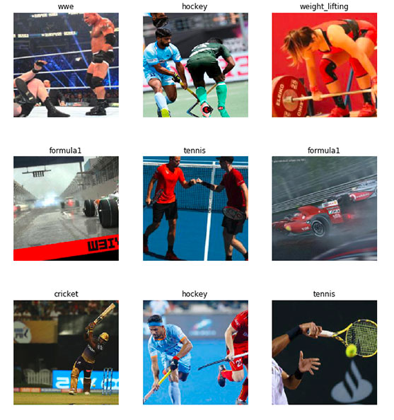
**图1：**由GitHub 用户使用Google 图片搜索策划的体育数据集"无足小视"。我们将使用此图像数据集与 Keras 进行视频分类。（图片来源)

我们今天在这里使用的数据集用于体育/活动分类。数据集由阿努巴夫·迈蒂策划，从谷歌图片下载照片（您也可以使用必应）为以下类别：

1. 游泳

2. 羽毛球

3. 摔跤

4. 奥运射击

5. 蟋蟀

6. 足球

7. 网球

8. 曲棍球

9. 冰球

10. 卡巴迪

11. WWE

12. 体育馆

13. 举重

14. 排球

15. 乒乓球

16. 棒球

17. 一级方程式

18. 摩托 GP

19. 棋

20. 拳击

21. 击剑

22. 篮球

为了节省时间、计算资源，并演示实际视频分类算法（本教程的实际点），我们将对运动类型数据集的子集进行培训：

• 足球（即足球）：799张图片
• 网球： 718 图片
• 举重： 577 图像

让我们继续下载我们的数据集！

项目结构

项目结构如下：

$ tree --dirsfirst --filelimit 50
.
├── Sports-Type-Classifier
│   ├── data
│   │   ├── football [799 entries]
│   │   ├── tennis [718 entries]
│   │   └── weight_lifting [577 entries]
├── example_clips
│   ├── lifting.mp4
│   ├── soccer.mp4
│   └── tennis.mp4
├── model
│   ├── activity.model
│   └── lb.pickle
├── output
├── plot.png
├── predict_video.py
└── train.py


  

 

  
1
  
2
  
3
  
4
  
5
  
6
  
7
  
8
  
9
  
10
  
11
  
12
  
13
  
14
  
15
  
16
  
17
  
18
  
19
 

我们的训练图像数据位于 Sports-Type-Classifier/data/ 目录中，按类别组织。

我从 YouTube 中为我们提取了三个 example_clips/ 来测试我们的模型。三个剪辑的积分位于“Keras 视频分类结果”部分的底部。

我们的分类器文件位于 model/ 目录中。包括 activity.model（经过训练的 Keras 模型）和 lb.pickle（我们的标签二值化器）。

一个空的 output/ 文件夹是我们将存储视频分类结果的位置。

我们将在今天的教程中介绍两个 Python 脚本：

• ​ train.py ：一个 Keras 训练脚本，它抓取我们关心的数据集类图像，加载 ResNet50 CNN，并应用 ImageNet 权重的转移学习/微调来训练我们的模型。训练脚本生成/输出三个文件：
  • model/activity.model ：基于 ResNet50 的微调分类器，用于识别运动。
  • model/lb.pickle ：包含我们独特的类标签的序列化标签二值化器。
  • plot.png ：准确率/损失训练历史图。
• predict_video.py ：从 example_clips/ 加载输入视频，然后使用今天的滚动平均方法对视频进行理想的分类。

实施我们的 Keras 培训脚本

让我们继续实施我们的训练脚本，用于训练Keras CNN来识别每一项体育活动。

打开train.py文件并插入以下代码：

# set the matplotlib backend so figures can be saved in the background
import matplotlib
matplotlib.use("Agg")
# import the necessary packages
from tensorflow.keras.preprocessing.image import ImageDataGenerator
from tensorflow.keras.layers import AveragePooling2D
from tensorflow.keras.applications import ResNet50
from tensorflow.keras.layers import Dropout
from tensorflow.keras.layers import Flatten
from tensorflow.keras.layers import Dense
from tensorflow.keras.layers import Input
from tensorflow.keras.models import Model
from tensorflow.keras.optimizers import SGD
from sklearn.preprocessing import LabelBinarizer
from sklearn.model_selection import train_test_split
from sklearn.metrics import classification_report
from imutils import paths
import matplotlib.pyplot as plt
import numpy as np
import argparse
import pickle
import cv2
import os

  

 

  
1
  
2
  
3
  
4
  
5
  
6
  
7
  
8
  
9
  
10
  
11
  
12
  
13
  
14
  
15
  
16
  
17
  
18
  
19
  
20
  
21
  
22
  
23
 

导入必要的包来训练我们的分类器：

matplotlib ：用于绘图。第 3 行设置后端，以便我们可以将训练图输出到 .png 图像文件。

tensorflow.keras：用于深度学习。也就是说，我们将使用 ResNet50 CNN。我们还将使用您可以在上周的教程中阅读的 ImageDataGenerator。

sklearn ：从 scikit-learn，我们将使用他们的 LabelBinarizer 实现来对我们的类标签进行单热编码。

train_test_split 函数将我们的数据集分割成训练和测试分割。我们还将以传统格式打印分类报告。

path ：包含用于列出给定路径中的所有图像文件的便利函数。从那里我们将能够将我们的图像加载到内存中。

numpy ：Python 的事实上的数值处理库。

argparse ：用于解析命令行参数。

pickle ：用于将我们的标签二值化器序列化到磁盘。

cv2：OpenCV。

os ：操作系统模块将用于确保我们获取与操作系统相关的正确文件/路径分隔符。

现在让我们继续解析我们的命令行参数：

# construct the argument parser and parse the arguments
ap = argparse.ArgumentParser()
ap.add_argument("-d", "--dataset", required=True,
	help="path to input dataset")
ap.add_argument("-m", "--model", required=True,
	help="path to output serialized model")
ap.add_argument("-l", "--label-bin", required=True,
	help="path to output label binarizer")
ap.add_argument("-e", "--epochs", type=int, default=25,
	help="# of epochs to train our network for")
ap.add_argument("-p", "--plot", type=str, default="plot.png",
	help="path to output loss/accuracy plot")
args = vars(ap.parse_args())

  

 

  
1
  
2
  
3
  
4
  
5
  
6
  
7
  
8
  
9
  
10
  
11
  
12
  
13
 

我们的脚本接受五个命令行参数，其中前三个是必需的：

–dataset ：输入数据集的路径。

–model ：我们输出 Keras 模型文件的路径。

–label-bin ：我们的输出标签二值化器pickle文件的路径。

–epochs ：我们的网络要训练多少个时期——默认情况下，我们将训练 25 个时期，但正如我将在本教程后面展示的，50 个时期可以带来更好的结果。

–plot ：我们的输出绘图图像文件的路径——默认情况下，它将被命名为 plot.png 并放置在与此训练脚本相同的目录中。

解析并掌握我们的命令行参数后，让我们继续初始化我们的 LABELS 并加载我们的数据：

# initialize the set of labels from the spots activity dataset we are
# going to train our network on
LABELS = set(["weight_lifting", "tennis", "football"])
# grab the list of images in our dataset directory, then initialize
# the list of data (i.e., images) and class images
print("[INFO] loading images...")
imagePaths = list(paths.list_images(args["dataset"]))
data = []
labels = []
# loop over the image paths
for imagePath in imagePaths:
	# extract the class label from the filename
	label = imagePath.split(os.path.sep)[-2]
	# if the label of the current image is not part of of the labels
	# are interested in, then ignore the image
	if label not in LABELS:
		continue
	# load the image, convert it to RGB channel ordering, and resize
	# it to be a fixed 224x224 pixels, ignoring aspect ratio
	image = cv2.imread(imagePath)
	image = cv2.cvtColor(image, cv2.COLOR_BGR2RGB)
	image = cv2.resize(image, (224, 224))
	# update the data and labels lists, respectively
	data.append(image)
	labels.append(label)

  

 

  
1
  
2
  
3
  
4
  
5
  
6
  
7
  
8
  
9
  
10
  
11
  
12
  
13
  
14
  
15
  
16
  
17
  
18
  
19
  
20
  
21
  
22
  
23
  
24
  
25
 

定义类 LABELS 的集合。该集合中不存在的所有标签都将被排除在我们的数据集之外。为了节省训练时间，我们的数据集将只包含举重、网球和足球/足球。通过对 LABELS 集进行更改，您可以随意使用其他类。

初始化我们的数据和标签列表。

遍历所有 imagePath。

在循环中，首先我们从 imagePath 中提取类标签

忽略不在 LABELS 集合中的任何标签。

加载并预处理图像。预处理包括将 OpenCV 的颜色通道交换到 Keras 兼容性并将大小调整为 224×224px。在此处阅读有关调整 CNN 图像大小的更多信息。要了解有关预处理重要性的更多信息，请务必参阅使用 Python 进行计算机视觉深度学习。

然后分别将图像和标签添加到数据和标签列表中。

继续，我们将对我们的标签进行单热编码并分区我们的数据：

# convert the data and labels to NumPy arrays
data = np.array(data)
labels = np.array(labels)
# perform one-hot encoding on the labels
lb = LabelBinarizer()
labels = lb.fit_transform(labels)
# partition the data into training and testing splits using 75% of
# the data for training and the remaining 25% for testing
(trainX, testX, trainY, testY) = train_test_split(data, labels,
	test_size=0.25, stratify=labels, random_state=42)

  

 

  
1
  
2
  
3
  
4
  
5
  
6
  
7
  
8
  
9
  
10
 

将我们的数据和标签列表转换为 NumPy 数组。

执行one-hot编码。one-hot编码是一种通过二进制数组元素标记活动类标签的方法。 例如，“足球”可能是 array([1, 0, 0]) 而“举重”可能是 array([0, 0, 1]) 。 请注意在任何给定时间只有一个类是“热的”。

按照4：1的比例，将我们的数据分成训练和测试部分。

初始化我们的数据增强对象：

# initialize the training data augmentation object
trainAug = ImageDataGenerator(
	rotation_range=30,
	zoom_range=0.15,
	width_shift_range=0.2,
	height_shift_range=0.2,
	shear_range=0.15,
	horizontal_flip=True,
	fill_mode="nearest")
# initialize the validation/testing data augmentation object (which
# we'll be adding mean subtraction to)
valAug = ImageDataGenerator()
# define the ImageNet mean subtraction (in RGB order) and set the
# the mean subtraction value for each of the data augmentation
# objects
mean = np.array([123.68, 116.779, 103.939], dtype="float32")
trainAug.mean = mean
valAug.mean = mean

  

 

  
1
  
2
  
3
  
4
  
5
  
6
  
7
  
8
  
9
  
10
  
11
  
12
  
13
  
14
  
15
  
16
  
17
  
18
 

初始化了两个数据增强对象——一个用于训练，一个用于验证。 在计算机视觉的深度学习中，几乎总是建议使用数据增强来提高模型泛化能力。

trainAug 对象对我们的数据执行随机旋转、缩放、移位、剪切和翻转。 您可以在此处阅读有关 ImageDataGenerator 和 fit 的更多信息。 正如我们上周强调的那样，请记住，使用 Keras，图像将即时生成（这不是附加操作）。

不会对验证数据 (valAug) 进行扩充，但我们将执行均值减法。

平均像素值，设置 trainAug 和 valAug 的均值属性，以便在训练/评估期间生成图像时进行均值减法。 现在，我们将执行我喜欢称之为“网络手术”的操作，作为微调的一部分：

# load the ResNet-50 network, ensuring the head FC layer sets are left
# off
baseModel = ResNet50(weights="imagenet", include_top=False,
	input_tensor=Input(shape=(224, 224, 3)))
# construct the head of the model that will be placed on top of the
# the base model
headModel = baseModel.output
headModel = AveragePooling2D(pool_size=(7, 7))(headModel)
headModel = Flatten(name="flatten")(headModel)
headModel = Dense(512, activation="relu")(headModel)
headModel = Dropout(0.5)(headModel)
headModel = Dense(len(lb.classes_), activation="softmax")(headModel)
# place the head FC model on top of the base model (this will become
# the actual model we will train)
model = Model(inputs=baseModel.input, outputs=headModel)
# loop over all layers in the base model and freeze them so they will
# *not* be updated during the training process
for layer in baseModel.layers:
	layer.trainable = False

  

 

  
1
  
2
  
3
  
4
  
5
  
6
  
7
  
8
  
9
  
10
  
11
  
12
  
13
  
14
  
15
  
16
  
17
  
18
  
19
 

加载用 ImageNet 权重预训练的 ResNet50，同时切掉网络的头部。

组装了一个新的 headModel 并将其缝合到 baseModel 上。

我们现在将冻结 baseModel，以便它不会通过反向传播进行训练。

让我们继续编译+训练我们的模型：

# compile our model (this needs to be done after our setting our
# layers to being non-trainable)
print("[INFO] compiling model...")
opt = SGD(lr=1e-4, momentum=0.9, decay=1e-4 / args["epochs"])
model.compile(loss="categorical_crossentropy", optimizer=opt,
	metrics=["accuracy"])
# train the head of the network for a few epochs (all other layers
# are frozen) -- this will allow the new FC layers to start to become
# initialized with actual "learned" values versus pure random
print("[INFO] training head...")
H = model.fit(
	x=trainAug.flow(trainX, trainY, batch_size=32),
	steps_per_epoch=len(trainX) // 32,
	validation_data=valAug.flow(testX, testY),
	validation_steps=len(testX) // 32,
	epochs=args["epochs"])

  

 

  
1
  
2
  
3
  
4
  
5
  
6
  
7
  
8
  
9
  
10
  
11
  
12
  
13
  
14
  
15
  
16
 

以前，TensorFlow/Keras 需要使用一种名为 .fit_generator 的方法来完成数据增强。现在，.fit 方法也可以处理数据增强，从而使代码更加一致。这也适用于从 .predict_generator 到 .predict 的迁移。请务必查看我关于 fit 和 fit_generator 以及数据增强的文章。

使用随机梯度下降 (SGD) 优化器编译我们的模型，初始学习率为 1e-4，学习率衰减。我们使用“categorical_crossentropy”损失来训练多类。如果您只使用两个类，请务必使用“binary_crossentropy”损失。

在我们的模型上调用 fit_generator 函数用数据增强和均值减法训练我们的网络。 请记住，我们的 baseModel 已冻结，我们只训练头部。这被称为“微调”。要快速了解微调，请务必阅读我之前的文章。要更深入地了解微调，请获取使用 Python 进行计算机视觉深度学习的 Practitioner Bundle 的副本。

我们将通过评估我们的网络并绘制训练历史来开始总结：

# evaluate the network
print("[INFO] evaluating network...")
predictions = model.predict(x=testX.astype("float32"), batch_size=32)
print(classification_report(testY.argmax(axis=1),
	predictions.argmax(axis=1), target_names=lb.classes_))
# plot the training loss and accuracy
N = args["epochs"]
plt.style.use("ggplot")
plt.figure()
plt.plot(np.arange(0, N), H.history["loss"], label="train_loss")
plt.plot(np.arange(0, N), H.history["val_loss"], label="val_loss")
plt.plot(np.arange(0, N), H.history["accuracy"], label="train_acc")
plt.plot(np.arange(0, N), H.history["val_accuracy"], label="val_acc")
plt.title("Training Loss and Accuracy on Dataset")
plt.xlabel("Epoch #")
plt.ylabel("Loss/Accuracy")
plt.legend(loc="lower left")
plt.savefig(args["plot"])

  

 

  
1
  
2
  
3
  
4
  
5
  
6
  
7
  
8
  
9
  
10
  
11
  
12
  
13
  
14
  
15
  
16
  
17
  
18
 

为了使此绘图片段与 TensorFlow 2+ 兼容，更新了 H.history 字典键以完全拼出“accuracy”无“acc”（H.history[“val_accuracy”] 和 H.历史[“准确性”]）。 “val”没有拼写为“validation”，这有点令人困惑； 我们必须学会热爱 API 并与之共存，并始终记住这是一项正在进行的工作，世界各地的许多开发人员都在为之做出贡献。

在我们在测试集上评估我们的网络并打印分类报告

之后，我们继续使用 matplotlib

绘制准确率/损失曲线。 该图通过第 164 行保存到磁盘。

最后将我们的模型和标签二值化器 (lb) 序列化到磁盘：

# serialize the model to disk
print("[INFO] serializing network...")
model.save(args["model"], save_format="h5")
# serialize the label binarizer to disk
f = open(args["label_bin"], "wb")
f.write(pickle.dumps(lb))
f.close()

  

 

  
1
  
2
  
3
  
4
  
5
  
6
  
7
 

训练结果

在我们 使用我们的 CNN 对视频中的帧进行分类，然后) 利用我们的 CNN 进行视频分类之前，我们首先需要训练模型。

确保您已使用本教程的“下载”部分将源代码下载到此图像（以及下载运动类型数据集）。

从那里，打开一个终端并执行以下命令：

$ python train.py --dataset Sports-Type-Classifier/data --model model/activity.model \
	--label-bin output/lb.pickle --epochs 50
[INFO] loading images...
[INFO] compiling model...
[INFO] training head...
Epoch 1/50
48/48 [==============================] - 10s 209ms/step - loss: 1.4184 - accuracy: 0.4421 - val_loss: 0.7866 - val_accuracy: 0.6719
Epoch 2/50
48/48 [==============================] - 10s 198ms/step - loss: 0.9002 - accuracy: 0.6086 - val_loss: 0.5476 - val_accuracy: 0.7832
Epoch 3/50
48/48 [==============================] - 9s 198ms/step - loss: 0.7188 - accuracy: 0.7020 - val_loss: 0.4690 - val_accuracy: 0.8105
Epoch 4/50
48/48 [==============================] - 10s 203ms/step - loss: 0.6421 - accuracy: 0.7375 - val_loss: 0.3986 - val_accuracy: 0.8516
Epoch 5/50
48/48 [==============================] - 10s 200ms/step - loss: 0.5496 - accuracy: 0.7770 - val_loss: 0.3599 - val_accuracy: 0.8652
...
Epoch 46/50
48/48 [==============================] - 9s 192ms/step - loss: 0.2066 - accuracy: 0.9217 - val_loss: 0.1618 - val_accuracy: 0.9336
Epoch 47/50
48/48 [==============================] - 9s 193ms/step - loss: 0.2064 - accuracy: 0.9204 - val_loss: 0.1622 - val_accuracy: 0.9355
Epoch 48/50
48/48 [==============================] - 9s 192ms/step - loss: 0.2092 - accuracy: 0.9217 - val_loss: 0.1604 - val_accuracy: 0.9375
Epoch 49/50
48/48 [==============================] - 9s 195ms/step - loss: 0.1935 - accuracy: 0.9290 - val_loss: 0.1620 - val_accuracy: 0.9375
Epoch 50/50
48/48 [==============================] - 9s 192ms/step - loss: 0.2109 - accuracy: 0.9164 - val_loss: 0.1561 - val_accuracy: 0.9395
[INFO] evaluating network...
                precision    recall  f1-score   support
      football       0.93      0.96      0.95       196
        tennis       0.92      0.92      0.92       179
weight_lifting       0.97      0.92      0.95       143
      accuracy                           0.94       518
     macro avg       0.94      0.94      0.94       518
  weighted avg       0.94      0.94      0.94       518
[INFO] serializing network...

  

 

  
1
  
2
  
3
  
4
  
5
  
6
  
7
  
8
  
9
  
10
  
11
  
12
  
13
  
14
  
15
  
16
  
17
  
18
  
19
  
20
  
21
  
22
  
23
  
24
  
25
  
26
  
27
  
28
  
29
  
30
  
31
  
32
  
33
  
34
  
35
 

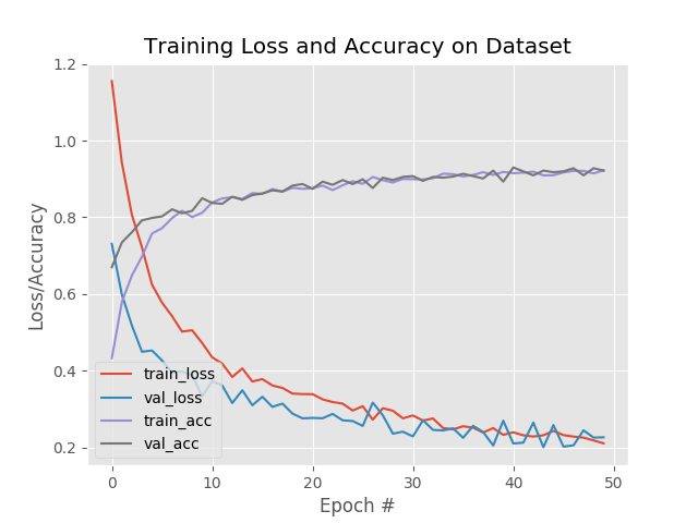
如您所见，在体育数据集上对 ResNet50 进行微调后，我们获得了约 94% 的准确率。 检查我们的模型目录，我们可以看到微调模型和标签二值化器已经序列化到磁盘：

使用 Keras 进行视频分类和滚动预测平均

我们现在准备通过滚动预测精度使用 Keras 实现视频分类！ 为了创建这个脚本，我们将利用视频的时间特性，特别是假设视频中的后续帧将具有相似的语义内容。 通过执行滚动预测准确性，我们将能够“平滑”预测并避免“预测闪烁”。 让我们开始吧——打开 predict_video.py 文件并插入以下代码：

# import the necessary packages
from tensorflow.keras.models import load_model
from collections import deque
import numpy as np
import argparse
import pickle
import cv2
# construct the argument parser and parse the arguments
ap = argparse.ArgumentParser()
ap.add_argument("-m", "--model", required=True,
	help="path to trained serialized model")
ap.add_argument("-l", "--label-bin", required=True,
	help="path to  label binarizer")
ap.add_argument("-i", "--input", required=True,
	help="path to our input video")
ap.add_argument("-o", "--output", required=True,
	help="path to our output video")
ap.add_argument("-s", "--size", type=int, default=128,
	help="size of queue for averaging")
args = vars(ap.parse_args())

  

 

  
1
  
2
  
3
  
4
  
5
  
6
  
7
  
8
  
9
  
10
  
11
  
12
  
13
  
14
  
15
  
16
  
17
  
18
  
19
  
20
 

加载必要的包和模块。 特别是，我们将使用 Python 集合模块中的 deque 来协助我们的滚动平均算法。

然后，解析五个命令行参数，其中四个是必需的：

–model ：从我们之前的训练步骤生成的输入模型的路径。

–label-bin ：前一个脚本生成的序列化 pickle 格式标签二值化器的路径。

–input ：用于视频分类的输入视频的路径。

–output ：我们将保存到磁盘的输出视频的路径。

–size ：滚动平均队列的最大大小（默认为 128）。 对于稍后的一些示例结果，我们将大小设置为 1，以便不执行平均。

有了我们的导入和命令行 args ，我们现在准备执行初始化：

# load the trained model and label binarizer from disk
print("[INFO] loading model and label binarizer...")
model = load_model(args["model"])
lb = pickle.loads(open(args["label_bin"], "rb").read())
# initialize the image mean for mean subtraction along with the
# predictions queue
mean = np.array([123.68, 116.779, 103.939][::1], dtype="float32")
Q = deque(maxlen=args["size"])

  

 

  
1
  
2
  
3
  
4
  
5
  
6
  
7
  
8
 

加载我们的模型和标签二值化器。

然后设置我们的平均减法值。 我们将使用双端队列来实现我们的滚动预测平均。

我们的双端队列 Q 使用等于 args[“size”] 值的 maxlen 初始化。

让我们初始化我们的 cv2.VideoCapture 对象并开始循环视频帧：

# initialize the video stream, pointer to output video file, and
# frame dimensions
vs = cv2.VideoCapture(args["input"])
writer = None
(W, H) = (None, None)
# loop over frames from the video file stream
while True:
	# read the next frame from the file
	(grabbed, frame) = vs.read()
	# if the frame was not grabbed, then we have reached the end
	# of the stream
	if not grabbed:
		break
	# if the frame dimensions are empty, grab them
	if W is None or H is None:
		(H, W) = frame.shape[:2]

  

 

  
1
  
2
  
3
  
4
  
5
  
6
  
7
  
8
  
9
  
10
  
11
  
12
  
13
  
14
  
15
  
16
 

抓取一个指向我们的输入视频文件流的指针。 我们使用 OpenCV 中的 VideoCapture 类从我们的视频流中读取帧。

然后，将我们的视频编写器和维度初始化为 None。

开始我们的视频分类 while 循环。

首先，我们抓取一个帧。 如果帧没有被抓取，那么我们已经到达了视频的结尾，此时我们将中断循环。

如果需要，然后设置我们的框架尺寸。 让我们预处理我们的框架：

# clone the output frame, then convert it from BGR to RGB
	# ordering, resize the frame to a fixed 224x224, and then
	# perform mean subtraction
	output = frame.copy()
	frame = cv2.cvtColor(frame, cv2.COLOR_BGR2RGB)
	frame = cv2.resize(frame, (224, 224)).astype("float32")
	frame -= mean

  

 

  
1
  
2
  
3
  
4
  
5
  
6
  
7
 

我们的框架副本用于输出目的。

然后，我们使用与训练脚本相同的步骤对帧进行预处理，包括：

​ 交换颜色通道。

​ 调整为 224×224px。

​ 平均减法。

接下来是帧分类推理和滚动预测平均：

# make predictions on the frame and then update the predictions
	# queue
	preds = model.predict(np.expand_dims(frame, axis=0))[0]
	Q.append(preds)
	# perform prediction averaging over the current history of
	# previous predictions
	results = np.array(Q).mean(axis=0)
	i = np.argmax(results)
	label = lb.classes_[i]

  

 

  
1
  
2
  
3
  
4
  
5
  
6
  
7
  
8
  
9
 

对当前帧进行预测。 预测结果通过第 64 行添加到 Q。

从那里，对 Q 历史执行预测平均，从而为滚动平均值生成一个类标签。 分解后，这些线在平均预测中找到具有最大对应概率的标签。

现在我们有了结果标签，让我们注释我们的输出帧并将其写入磁盘：

# draw the activity on the output frame
	text = "activity: {}".format(label)
	cv2.putText(output, text, (35, 50), cv2.FONT_HERSHEY_SIMPLEX,
		1.25, (0, 255, 0), 5)
	# check if the video writer is None
	if writer is None:
		# initialize our video writer
		fourcc = cv2.VideoWriter_fourcc(*"MJPG")
		writer = cv2.VideoWriter(args["output"], fourcc, 30,
			(W, H), True)
	# write the output frame to disk
	writer.write(output)
	# show the output image
	cv2.imshow("Output", output)
	key = cv2.waitKey(1) & 0xFF
	# if the `q` key was pressed, break from the loop
	if key == ord("q"):
		break
# release the file pointers
print("[INFO] cleaning up...")
writer.release()
vs.release()

  

 

  
1
  
2
  
3
  
4
  
5
  
6
  
7
  
8
  
9
  
10
  
11
  
12
  
13
  
14
  
15
  
16
  
17
  
18
  
19
  
20
  
21
  
22
 

在输出帧上绘制预测。

如有必要，初始化视频编写器。 输出帧被写入文件（第 85 行）。 在此处阅读有关使用 OpenCV 写入视频文件的更多信息。

输出也显示在屏幕上，直到按下 q 键（或如上所述到达视频文件的末尾）。

最后，我们将执行清理。

Keras 视频分类结果

现在我们已经使用 Keras 实现了我们的视频分类器，让我们将其投入使用。

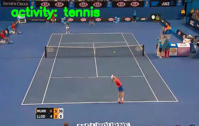
让我们将视频分类应用于“网球”剪辑——但让我们将队列的 --size 设置为 1，轻松地将视频分类转换为标准图像分类：

$ python predict_video.py --model model/activity.model \
	--label-bin model/lb.pickle \
	--input example_clips/tennis.mp4 \
	--output output/tennis_1frame.avi \
	--size 1
Using TensorFlow backend.
[INFO] loading model and label binarizer...
[INFO] cleaning up...

  

 

  
1
  
2
  
3
  
4
  
5
  
6
  
7
  
8
 

Video classification with Keras and Deep Learning - PyImageSearch

正如你所看到的，有相当多的标签闪烁——我们的 CNN 认为某些帧是“网球”（正确）而其他帧是“足球”（不正确）。

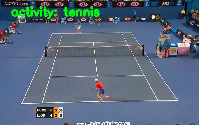
现在让我们使用默认队列 --size 128，从而利用我们的预测平均算法来平滑结果：

$ python predict_video.py --model model/activity.model \
	--label-bin model/lb.pickle \
	--input example_clips/tennis.mp4 \
	--output output/tennis_128frames_smoothened.avi \
	--size 128
Using TensorFlow backend.
[INFO] loading model and label binarizer...
[INFO] cleaning up...

  

 

  
1
  
2
  
3
  
4
  
5
  
6
  
7
  
8
 

Video classification with Keras and Deep Learning - PyImageSearch

请注意我们如何正确地将此视频标记为“网球”！

在以后的教程中，我们将介绍更高级的活动和视频分类方法，包括 LSTM 和 RNN。

总结

在本教程中，您学习了如何使用 Keras 和深度学习执行视频分类。

一种简单的视频分类算法是将视频的每一帧视为独立于其他帧。这种类型的实现会导致“标签闪烁”，即 CNN 为后续帧返回不同的标签，即使这些帧应该是相同的标签！

更高级的神经网络，包括 LSTM 和更通用的 RNN，可以帮助解决这个问题并带来更高的准确性。然而，LSTMs 和 RNNs 可能会根据你正在做的事情产生戏剧性的矫枉过正——在某些情况下，简单的滚动预测平均会给你带来你需要的结果。

使用滚动预测平均，您可以维护来自 CNN 的最后 K 个预测的列表。然后我们取这最后 K 个预测，对它们求平均，选择概率最大的标签，然后选择这个标签对当前帧进行分类。这里的假设是视频中的后续帧将具有相似的语义内容。

如果这个假设成立，那么我们可以利用视频的时间特性，假设前一帧与当前帧相似。 因此，平均使我们能够平滑预测并形成更好的视频分类器。

在以后的教程中，我们还将讨论更高级的 LSTM 和 RNN。

文章来源: wanghao.blog.csdn.net，作者：AI浩，版权归原作者所有，如需转载，请联系作者。

原文链接：wanghao.blog.csdn.net/article/details/121044209