使用Tensorflow ，完成CIFAR-10图像识别，作者：北山啦

数据集官网：The CIFAR-10 dataset

@[toc]

import warnings
warnings.filterwarnings('ignore')
import tensorflow as tf
import matplotlib.pyplot as plt
import os 
import numpy as np
%matplotlib inline

• CIFAR-10是一个更接近普适物体的彩色图像数据集。CIFAR-10 是由Hinton 的学生Alex Krizhevsky 和Ilya Sutskever 整理的一个用于识别普适物体的小型数据集。一共包含10 个类别的RGB 彩色图片：飞机（ airplane ）、汽车（ automobile ）、鸟类（ bird ）、猫（ cat ）、鹿（ deer ）、狗（ dog ）、蛙类（ frog ）、马（ horse ）、船（ ship ）和卡车（ truck ）。

• 每个图片的尺寸为32 × 32 ，每个类别有6000个图像，数据集中一共有50000 张训练图片和10000 张测试图片。

数据集介绍

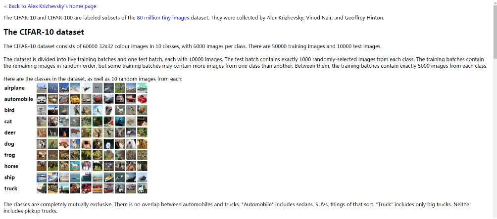
• CIFAR-10是一个用于识别普适物 体的小型数据集，它包含了10个类 别的RGB彩色图片。
• 图片尺寸： 32 x 32
• 训练图片50000张，测试图片 10000张

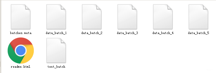
导入CIFAR数据集

def load_CIFAR_batch(filename):
    with open(filename,"rb") as f:
        data_dict = np.load(f,encoding="bytes", allow_pickle=True)
        images = data_dict[b"data"]
        labels = data_dict[b"labels"]
        images = images.reshape(10000,3,32,32)
        images = images.transpose(0,2,3,1)
        labels = np.array(labels)
        return images,labels

def load_CIFAR_data(data_dir):
    images_train=[]
    labels_train=[]
    for i in range(5):
        f = os.path.join(data_dir,"data_batch_%d"%(i+1))
        print("正在加载",f)
        image_batch,label_batch = load_CIFAR_batch(f)
        images_train.append(image_batch)
        labels_train.append(label_batch)
        Xtrain = np.concatenate(images_train)
        Ytrain = np.concatenate(labels_train)
        del image_batch,label_batch
    Xtest,Ytest = load_CIFAR_batch(os.path.join(data_dir,"test_batch"))
    print("导入完成")
    
    return Xtrain,Ytrain,Xtest,Ytest

data_dir = r"data\cifar-10-batches-py"
Xtrain,Ytrain,Xtest,Ytest = load_CIFAR_data(data_dir)

正在加载 data\cifar-10-batches-py\data_batch_1
正在加载 data\cifar-10-batches-py\data_batch_2
正在加载 data\cifar-10-batches-py\data_batch_3
正在加载 data\cifar-10-batches-py\data_batch_4
正在加载 data\cifar-10-batches-py\data_batch_5
导入完成

显示数据集信息

print("training data shpae:\t",Xtrain.shape)
print("training labels shpae:\t",Ytrain.shape)
print("test data shpae:\t",Xtest.shape)
print("test labels shpae:\t",Ytest.shape)

training data shpae:	 (50000, 32, 32, 3)
training labels shpae:	 (50000,)
test data shpae:	 (10000, 32, 32, 3)
test labels shpae:	 (10000,)

Ytest

array([3, 8, 8, ..., 5, 1, 7])

查看image和label

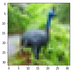
查看单项image

plt.imshow(Xtrain[6])

<matplotlib.image.AxesImage at 0xb7b5e48>

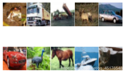
查看多项images

for i in range(0,10):
    fig = plt.gcf()
    fig.set_size_inches(12,6)
    ax = plt.subplot(2,5,i+1)
    # 去除坐标轴
    plt.xticks([])
    plt.yticks([])

    # 去除黑框
    ax.spines['top'].set_visible(False)
    ax.spines['right'].set_visible(False)
    ax.spines['bottom'].set_visible(False)
    ax.spines['left'].set_visible(False)
    # 设置各个子图间间距
    plt.subplots_adjust(left=0.10, top=0.88, right=0.65, bottom=0.08, wspace=0.02, hspace=0.02)
    ax.imshow(Xtrain[i],cmap="binary")

查看多项iamges和label

label_dict  = {0:"airplane",1:"automobile",2:"bird",3:"cat",4:"deer",5:"dog",6:"frog",7:"horse",8:"ship",9:"trunk"}

def plot_images_labels_prediction(images,labels,prediction,idx,num=10):
    fig = plt.gcf()
    fig.set_size_inches(12,6)
    if num >10:
        num=10
        
    for i in range(0,num):
        ax = plt.subplot(2,5,i+1)
        ax.imshow(images[idx],cmap="binary")
        plt.xticks([])
        plt.yticks([])

        # 去除黑框
        ax.spines['top'].set_visible(False)
        ax.spines['right'].set_visible(False)
        ax.spines['bottom'].set_visible(False)
        ax.spines['left'].set_visible(False)
        title = str(i)+","+label_dict[labels[idx]]
        if len(prediction)>0:
            title+="=>"+label_dict[prediction[idx]]
        ax.set_title(title,fontsize=10)
        idx += 1
        # 去除坐标轴

    plt.show()

plot_images_labels_prediction(Xtest,Ytest,[],1,10)

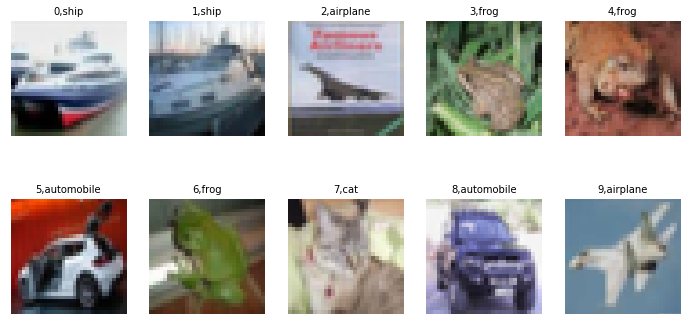
定义网络结构

• 图像的特征提取：通过卷基层1、降采样层1、卷积层2以及降采样层2的处理，提取网络结构
• 全连接神经网络：全连接层、输出层所组成的网络结构

图像的预处理

查看那图像数据信息
显示第一个图的第一个像素点

Xtrain[0][0][0]

array([59, 62, 63], dtype=uint8)

将图像进行数字的标准化

Xtrain_normalize = Xtrain.astype("float32")/255.0
Xtest_normalize = Xtest.astype("float32")/255.0

查看预处理后图像数据信息

Xtrain_normalize[0][0][0]

array([ 0.23137255,  0.24313726,  0.24705882], dtype=float32)

标签数据预处理–独热编码

1. 能够处理非连续型数值特征
2. 在一定程度上也扩充了特征

from sklearn.preprocessing import OneHotEncoder

encoder = OneHotEncoder(sparse=False)
yy = [[0],[1],[2],[3],[4],[5],[6],[7],[8],[9]]
encoder.fit(yy)
Ytrain_reshape = Ytrain.reshape(-1,1)
Ytrain_onehot = encoder.transform(Ytrain_reshape)
Ytest_reshape = Ytest.reshape(-1,1)
Ytest_onehot = encoder.transform(Ytest_reshape)

Ytrain[:10]

array([6, 9, 9, 4, 1, 1, 2, 7, 8, 3])

Ytrain_onehot.shape

(50000, 10)

Ytrain[:5]

array([6, 9, 9, 4, 1])

Ytrain_onehot[:5]

array([[ 0.,  0.,  0.,  0.,  0.,  0.,  1.,  0.,  0.,  0.],
       [ 0.,  0.,  0.,  0.,  0.,  0.,  0.,  0.,  0.,  1.],
       [ 0.,  0.,  0.,  0.,  0.,  0.,  0.,  0.,  0.,  1.],
       [ 0.,  0.,  0.,  0.,  1.,  0.,  0.,  0.,  0.,  0.],
       [ 0.,  1.,  0.,  0.,  0.,  0.,  0.,  0.,  0.,  0.]])

定义共享函数

# 定义权值
def weight(shape):
    # 在构建模型时，需要用tf.Variable来创建一个变量
    # 再训练时，这个变量不断更新
    # 使用函数tf.truncated_normal(截断的正太分布)生成标准差为0.1的随机数来初始化权值
    return tf.Variable(tf.truncated_normal(shape,stddev=0.1),name="W")


# 定义偏置，初始值为0.1
def bias(shape):
    return tf.Variable(tf.constant(0.1,shape=shape),name="b")



# 定义卷积操作，步长为1，padding为same
def conv2d(x,W):
    return tf.nn.conv2d(x,W,strides=[1,1,1,1],padding="SAME")



# 定义池化操作
# 步长为2，即原尺寸的长和宽各除以2
def max_pool_2x2(x):
    return tf.nn.max_pool(x,ksize=[1,2,2,1],strides=[1,2,2,1],padding="SAME")

定义网络结构

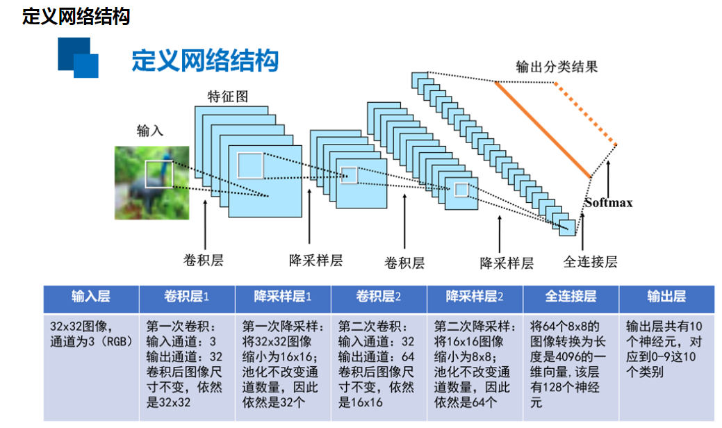
==图像的特征提取==：通过卷积层1，降采样层1，卷积层2以及降 采样层2的处理，提取图像的特征

==全连接神经网络==：全连接层、输出层所组成的网络结构

"""输入层，32*32图像，通道为3RGB"""

with tf.name_scope("input_layer"):
    x = tf.placeholder("float",shape=[None,32,32,3],name="x")

"""第一个卷积层"""    
with tf.name_scope("conv_1"):
    W1 = weight([3,3,3,32])
    b1 = bias([32])
    conv_1 = conv2d(x,W1)+b1
    conv_1 = tf.nn.relu(conv_1)
"""第一个池化层"""
with tf.name_scope("pool_1"):
    pool_1 = max_pool_2x2(conv_1)
"""第一个卷积层"""    
with tf.name_scope("conv_2"):
    W2 = weight([3,3,32,64])
    b2 = bias([64])
    conv_2 = conv2d(pool_1,W2)+b2
    conv_2  = tf.nn.relu(conv_2)

"""第二个池化层"""
with tf.name_scope("pool_2"):
    pool_2 = max_pool_2x2(conv_2)
with tf.name_scope("fc"):
    W3 = weight([4096,128])
    b3 = bias([128])
    flat = tf.reshape(pool_2,[-1,4096])
    h = tf.nn.relu(tf.matmul(flat,W3)+b3)
    h_dropout = tf.nn.dropout(h,keep_prob=0.8)

with tf.name_scope("output_layer"):
    W4 = weight([128,10])
    b4 = bias([10])
    pred = tf.nn.softmax(tf.matmul(h_dropout,W4)+b4)

构建模型

with tf.name_scope("optimizer"):
    y = tf.placeholder("float",shape=[None,10],name ="label")
    loss_function = tf.reduce_mean(tf.nn.softmax_cross_entropy_with_logits(logits=pred,labels=y))
    optimizer = tf.train.AdamOptimizer(learning_rate=0.0001).minimize(loss_function)

定义准确率

with tf.name_scope("evaluation"):
    correct_prediction = tf.equal(tf.argmax(pred,1),tf.argmax(y,1))
    accuracy = tf.reduce_mean(tf.cast(correct_prediction,"float"))

启动会话

import os 
from time import time
train_epochs = 25
batch_size = 50
total_batch = int(len(Xtrain)/batch_size)
epoch_list=[]
accuracy_list = []
loss_list=[];
epoch = tf.Variable(0,name="epoch",trainable=False)
startTime = time()
sess  =tf.Session()
init = tf.global_variables_initializer()
sess.run(init)

断点续训

ckpt_dir = "CIFAR10_log/"
if not os.path.exists(ckpt_dir):
    os.makedirs(ckpt_dir)
saver = tf.train.Saver(max_to_keep=1)
ckpt = tf.train.latest_checkpoint(ckpt_dir)
if ckpt != None:
    saver.restore(sess,ckpt)
else:
    print("Training from search")
start = sess.run(epoch)
print("Training starts from {} epoch".format(start+1))

Training from search
Training starts from 1 epoch

迭代训练

def get_train_batch(number, batch_size):
    return Xtrain_normalize[number*batch_size:(number+1)*batch_size],Ytrain_onehot[number*batch_size:(number+1)*batch_size]
for ep in range(start, train_epochs):
    for i in range(total_batch):
        batch_x,batch_y = get_train_batch(i,batch_size)
        sess.run(optimizer, feed_dict= {x:batch_x, y:batch_y})
        if i % 100 == 0:
            print("Step {}".format(i), "finished")
    loss,acc = sess.run([loss_function,accuracy],feed_dict={x: batch_x, y: batch_y})
    epoch_list.append(ep+1)
    loss_list.append(loss)
    accuracy_list.append(acc)
    print("Train epoch:", "%02d" % (sess.run(epoch)+1),"Loss=","{:.6f}".format(loss),"Accuracy=",acc)#保存检查点
    saver.save(sess,ckpt_dir+"CIFAR10_cnn_model.cpkt",global_step=ep+1)
    sess.run(epoch.assign(ep+1))
duration =time()-startTime
print("Train finished takes:",duration)

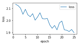
可视化损失

fig = plt.gcf()
fig.set_size_inches(4,2)
plt.plot(epoch_list,loss_list,label="loss")
plt.ylabel("loss")
plt.xlabel("epoch")
plt.legend(["loss"],loc="best")

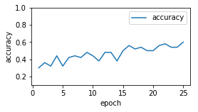
可视化准确率

plt.plot(epoch_list,accuracy_list,label="accuracy")
fig = plt.gcf()
fig.set_size_inches(4,2)
plt.ylim(0.1,1)
plt.ylabel("accuracy")
plt.xlabel("epoch")
plt.legend()
plt.show()

评估模型及预测

test_total_batch = int(len(Xtest_normalize)/batch_size)
test_acc_sum = 0.0
for i in range(test_total_batch):
    test_image_batch = Xtest_normalize[i*batch_size(i+1)*batch_size]
    test_label_batch = Ytest_onehot[i*batch_size:(i+1)*batch_size]
    test_batch_acc = sess.run(accuracy,feed_dict={x:test_image_batch,y:test_label_batch})
    test_acc_sum += test_batch_acc
test_acc = float(test_acc_sum/test_total_batch)
print("Test accuracy:{:.6f}".format(test_acc))

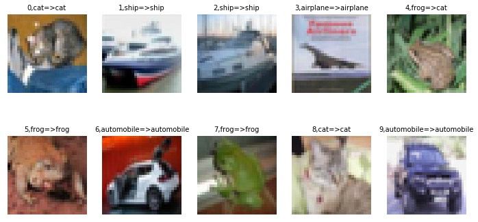
test_pred = sess.run(pred,feed_dict={x:Xtest_normalize[:10]})
prediction_result = sess.run(tf.argmax(test_pred,1))

plot_images_labels_prediction(Xtest,Ytest,prediction_result,0,10)

到这里就结束了，如果对你有帮助，欢迎点赞关注评论，你的点赞对我很重要，author：北山啦