基于三阶贝塞尔曲线的数据平滑算法

前言
很多文章在谈及曲线平滑的时候,习惯使用拟合的概念,我认为这是不恰当的。平滑后的曲线,一定经过原始的数据点,而拟合曲线,则不一定要经过原始数据点。
一般而言,需要平滑的数据分为两种:时间序列的单值数据、时间序列的二维数据。对于前者,并非一定要用贝塞尔算法,仅用样条插值就可以轻松实现平滑;而对于后者,不管是 numpy 还是 scipy 提供的那些插值算法,就都不适用了。
本文基于三阶贝塞尔曲线,实现了时间序列的单值数据和时间序列的二维数据的平滑算法,可满足大多数的平滑需求。
贝塞尔曲线
关于贝塞尔曲线的数学原理,这里就不讨论了,直接贴出结论:
-
一阶贝塞尔曲线

-
二阶贝塞尔曲线
-
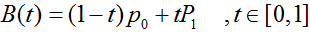
三阶贝塞尔曲线


算法描述
如果我们把三阶贝塞尔曲线的 P0 和 P3 视为原始数据,只要找到 P1 和 P2 两个点(我们称其为控制点),就可以根据三阶贝塞尔曲线公式,计算出 P0 和 P3 之间平滑曲线上的任意点。
现在,平滑问题变成了如何计算两个原始数据点之间的控制点的问题。步骤如下:
第1步:绿色直线连接相邻的原始数据点,计算出个线段的中点,红色直线连接相邻的中点
第2步:根据相邻两条绿色直线长度之比,分割其中点之间红色连线,标记分割点
第3步:平移红色连线,使其分割点与相对的原始数据点重合
第4步:调整平移后红色连线的端点与原始数据点的距离,通常缩减40%-80%
算法实现
# -*- coding: utf-8 -*-
import numpy as np
def bezier_curve(p0, p1, p2, p3, inserted): """ 三阶贝塞尔曲线 p0, p1, p2, p3 - 点坐标,tuple、list或numpy.ndarray类型 inserted - p0和p3之间插值的数量 """ assert isinstance(p0, (tuple, list, np.ndarray)), u'点坐标不是期望的元组、列表或numpy数组类型' assert isinstance(p0, (tuple, list, np.ndarray)), u'点坐标不是期望的元组、列表或numpy数组类型' assert isinstance(p0, (tuple, list, np.ndarray)), u'点坐标不是期望的元组、列表或numpy数组类型' assert isinstance(p0, (tuple, list, np.ndarray)), u'点坐标不是期望的元组、列表或numpy数组类型' if isinstance(p0, (tuple, list)): p0 = np.array(p0) if isinstance(p1, (tuple, list)): p1 = np.array(p1) if isinstance(p2, (tuple, list)): p2 = np.array(p2) if isinstance(p3, (tuple, list)): p3 = np.array(p3) points = list() for t in np.linspace(0, 1, inserted+2): points.append(p0*np.power((1-t),3) + 3*p1*t*np.power((1-t),2) + 3*p2*(1-t)*np.power(t,2) + p3*np.power(t,3)) return np.vstack(points)
def smoothing_base_bezier(date_x, date_y, k=0.5, inserted=10, closed=False): """ 基于三阶贝塞尔曲线的数据平滑算法 date_x - x维度数据集,list或numpy.ndarray类型 date_y - y维度数据集,list或numpy.ndarray类型 k - 调整平滑曲线形状的因子,取值一般在0.2~0.6之间。默认值为0.5 inserted - 两个原始数据点之间插值的数量。默认值为10 closed - 曲线是否封闭,如是,则首尾相连。默认曲线不封闭 """ assert isinstance(date_x, (list, np.ndarray)), u'x数据集不是期望的列表或numpy数组类型' assert isinstance(date_y, (list, np.ndarray)), u'y数据集不是期望的列表或numpy数组类型' if isinstance(date_x, list) and isinstance(date_y, list): assert len(date_x)==len(date_y), u'x数据集和y数据集长度不匹配' date_x = np.array(date_x) date_y = np.array(date_y) elif isinstance(date_x, np.ndarray) and isinstance(date_y, np.ndarray): assert date_x.shape==date_y.shape, u'x数据集和y数据集长度不匹配' else: raise Exception(u'x数据集或y数据集类型错误') # 第1步:生成原始数据折线中点集 mid_points = list() for i in range(1, date_x.shape[0]): mid_points.append({ 'start': (date_x[i-1], date_y[i-1]), 'end': (date_x[i], date_y[i]), 'mid': ((date_x[i]+date_x[i-1])/2.0, (date_y[i]+date_y[i-1])/2.0) }) if closed: mid_points.append({ 'start': (date_x[-1], date_y[-1]), 'end': (date_x[0], date_y[0]), 'mid': ((date_x[0]+date_x[-1])/2.0, (date_y[0]+date_y[-1])/2.0) }) # 第2步:找出中点连线及其分割点 split_points = list() for i in range(len(mid_points)): if i < (len(mid_points)-1): j = i+1 elif closed: j = 0 else: continue x00, y00 = mid_points[i]['start'] x01, y01 = mid_points[i]['end'] x10, y10 = mid_points[j]['start'] x11, y11 = mid_points[j]['end'] d0 = np.sqrt(np.power((x00-x01), 2) + np.power((y00-y01), 2)) d1 = np.sqrt(np.power((x10-x11), 2) + np.power((y10-y11), 2)) k_split = 1.0*d0/(d0+d1) mx0, my0 = mid_points[i]['mid'] mx1, my1 = mid_points[j]['mid'] split_points.append({ 'start': (mx0, my0), 'end': (mx1, my1), 'split': (mx0+(mx1-mx0)*k_split, my0+(my1-my0)*k_split) }) # 第3步:平移中点连线,调整端点,生成控制点 crt_points = list() for i in range(len(split_points)): vx, vy = mid_points[i]['end'] # 当前顶点的坐标 dx = vx - split_points[i]['split'][0] # 平移线段x偏移量 dy = vy - split_points[i]['split'][1] # 平移线段y偏移量 sx, sy = split_points[i]['start'][0]+dx, split_points[i]['start'][1]+dy # 平移后线段起点坐标 ex, ey = split_points[i]['end'][0]+dx, split_points[i]['end'][1]+dy # 平移后线段终点坐标 cp0 = sx+(vx-sx)*k, sy+(vy-sy)*k # 控制点坐标 cp1 = ex+(vx-ex)*k, ey+(vy-ey)*k # 控制点坐标 if crt_points: crt_points[-1].insert(2, cp0) else: crt_points.append([mid_points[0]['start'], cp0, mid_points[0]['end']]) if closed: if i < (len(mid_points)-1): crt_points.append([mid_points[i+1]['start'], cp1, mid_points[i+1]['end']]) else: crt_points[0].insert(1, cp1) else: if i < (len(mid_points)-2): crt_points.append([mid_points[i+1]['start'], cp1, mid_points[i+1]['end']]) else: crt_points.append([mid_points[i+1]['start'], cp1, mid_points[i+1]['end'], mid_points[i+1]['end']]) crt_points[0].insert(1, mid_points[0]['start']) # 第4步:应用贝塞尔曲线方程插值 out = list() for item in crt_points: group = bezier_curve(item[0], item[1], item[2], item[3], inserted) out.append(group[:-1]) out.append(group[-1:]) out = np.vstack(out) return out.T[0], out.T[1]
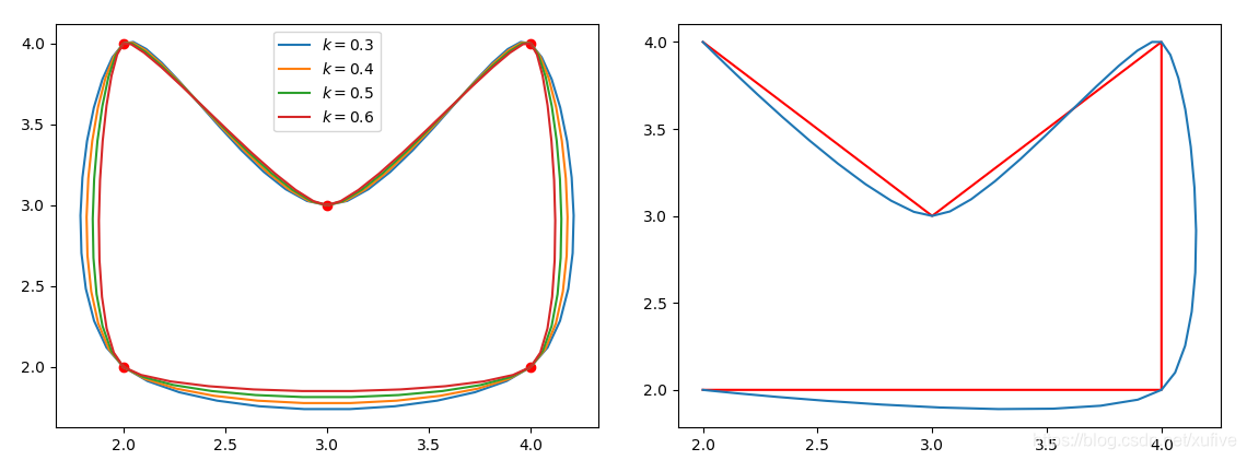
if __name__ == '__main__': import matplotlib.pyplot as plt x = np.array([2,4,4,3,2]) y = np.array([2,2,4,3,4]) plt.plot(x, y, 'ro') x_curve, y_curve = smoothing_base_bezier(x, y, k=0.3, closed=True) plt.plot(x_curve, y_curve, label='$k=0.3$') x_curve, y_curve = smoothing_base_bezier(x, y, k=0.4, closed=True) plt.plot(x_curve, y_curve, label='$k=0.4$') x_curve, y_curve = smoothing_base_bezier(x, y, k=0.5, closed=True) plt.plot(x_curve, y_curve, label='$k=0.5$') x_curve, y_curve = smoothing_base_bezier(x, y, k=0.6, closed=True) plt.plot(x_curve, y_curve, label='$k=0.6$') plt.legend(loc='best') plt.show()
- 1
- 2
- 3
- 4
- 5
- 6
- 7
- 8
- 9
- 10
- 11
- 12
- 13
- 14
- 15
- 16
- 17
- 18
- 19
- 20
- 21
- 22
- 23
- 24
- 25
- 26
- 27
- 28
- 29
- 30
- 31
- 32
- 33
- 34
- 35
- 36
- 37
- 38
- 39
- 40
- 41
- 42
- 43
- 44
- 45
- 46
- 47
- 48
- 49
- 50
- 51
- 52
- 53
- 54
- 55
- 56
- 57
- 58
- 59
- 60
- 61
- 62
- 63
- 64
- 65
- 66
- 67
- 68
- 69
- 70
- 71
- 72
- 73
- 74
- 75
- 76
- 77
- 78
- 79
- 80
- 81
- 82
- 83
- 84
- 85
- 86
- 87
- 88
- 89
- 90
- 91
- 92
- 93
- 94
- 95
- 96
- 97
- 98
- 99
- 100
- 101
- 102
- 103
- 104
- 105
- 106
- 107
- 108
- 109
- 110
- 111
- 112
- 113
- 114
- 115
- 116
- 117
- 118
- 119
- 120
- 121
- 122
- 123
- 124
- 125
- 126
- 127
- 128
- 129
- 130
- 131
- 132
- 133
- 134
- 135
- 136
- 137
- 138
- 139
- 140
- 141
- 142
- 143
- 144
- 145
- 146
- 147
- 148
- 149
- 150
- 151
- 152
- 153
- 154
- 155
- 156
- 157
- 158
- 159
下图为平滑效果。左侧是封闭曲线,两个原始数据点之间插值数量为默认值10;右侧为同样数据不封闭的效果,k值默认0.5.
参考资料
算法参考了 Interpolation with Bezier Curves 这个网页,里面没有关于作者的任何信息,在此只能笼统地向国际友人表示感谢!
文章来源: xufive.blog.csdn.net,作者:天元浪子,版权归原作者所有,如需转载,请联系作者。
原文链接:xufive.blog.csdn.net/article/details/86163741

- 点赞
- 收藏
- 关注作者
评论(0)