神经网络--从0开始搭建过拟合和防过拟合模型


前言:Hello大家好,我是Dream。 今天来学习一下如何从0开始搭建过拟合和防过拟合模型,本文是从零开始的,如有需要可自行跳至所需内容~
@TOC
说明:在此试验下,我们使用的是使用tf2.x版本,在jupyter环境下完成
在本文中,我们将主要完成以下任务:
-
加载keras内置的fashion mnist数据库
-
自己搭建任意神经网络,并自选损失函数和优化方法
-
可以使用防止过拟合的任何手段,要通过对比方法证明手段有效
-
训练和评估的准确率以及损失函数,要以图表形式显示
一、Fashion-MNIST数据集简介
1.数据库内容
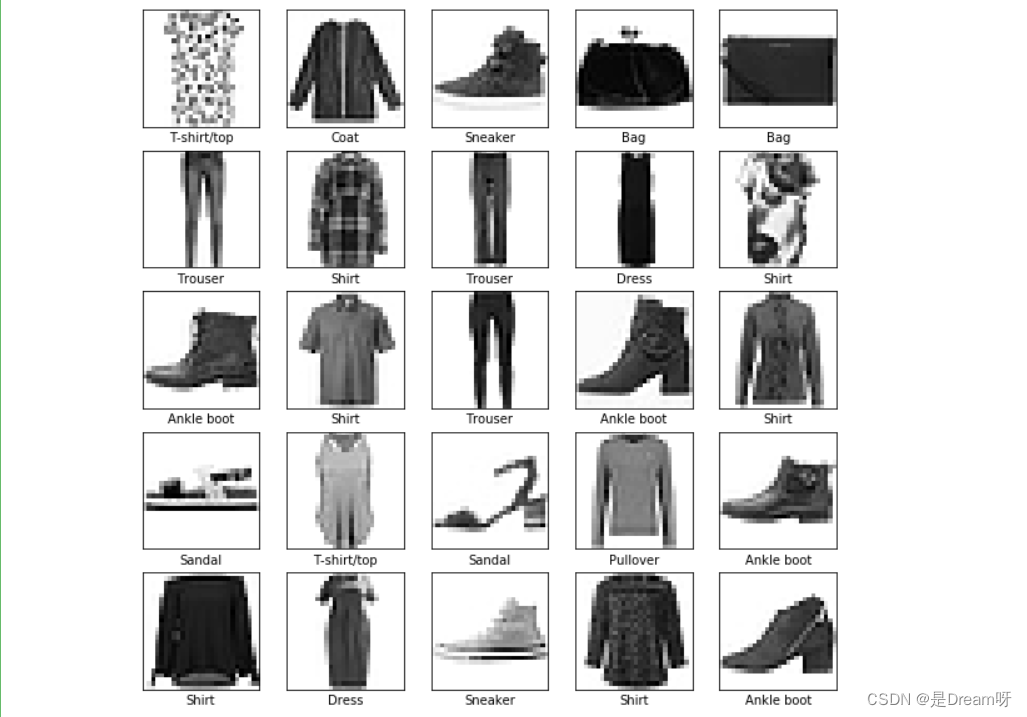
Fashion-MNIST数据集包含了10个类别的图像,分别是:t-shirt(T恤),trouser(牛仔裤),pullover(套衫),dress(裙子),coat(外套),sandal(凉鞋),shirt(衬衫),sneaker(运动鞋),bag(包),ankle boot(短靴)
2.数据量
我们可以用len()来获取该数据集的大小,还可以用下标来获取具体的一个样本。训练集和测试机中的每一个类别的图像数分别为6000和1000。因为有10个类别,所以训练集和测试集的样本数分别为60000和10000。#数据集大小 print(len(mnist_train), len(mnist_test))
3.数据及标签的具体形式
每个样本均为28x28大小(即共有784个像素)的单通道灰度图,并由10种类别通过0-9数字进行标记;
10种类别分别是:
0 T-shirt/top
1 Trouser
2 Pullover
3 Dress
4 Coat
5 Sandal
6 Shirt
7 Sneaker
8 Bag
9 Ankle boot
4.显示随机数据样本及对应标签
import tensorflow as tf
import matplotlib.pyplot as plt
import numpy as np
# 指定当前程序使用的 GPU
gpus = tf.config.experimental.list_physical_devices('GPU')
for gpu in gpus:
    tf.config.experimental.set_memory_growth(gpu, True)
# 调用数据集
(train_X, train_y), (test_X, test_y) = tf.keras.datasets.fashion_mnist.load_data()
train_X, test_X = train_X / 255.0, test_X / 255.0
class_names = ['T-shirt/top', 'Trouser', 'Pullover', 'Dress', 'Coat',
               'Sandal', 'Shirt', 'Sneaker', 'Bag', 'Ankle boot']

plt.figure(figsize=(10, 10))
place = 0
for i in np.random.randint(1, 10000, 25):
    plt.subplot(5, 5, place+1)
    place += 1
    plt.xticks([])
    plt.yticks([])
    plt.grid(False)
    plt.imshow(train_X[i], cmap=plt.cm.binary)
    plt.xlabel(class_names[train_y[i]])
plt.show()
🌟🌟🌟这里是输出的结果:✨✨✨
二、过拟合模型
1.调用库函数
import tensorflow as tf
import matplotlib.pyplot as plt
from sklearn.model_selection import train_test_split
from tensorflow.keras.preprocessing.image import ImageDataGenerator
from tensorflow.keras.layers import Conv2D,MaxPooling2D,BatchNormalization,Flatten,Dense,Dropout
# 指定当前程序使用的 GPU
gpus = tf.config.experimental.list_physical_devices('GPU')
for gpu in gpus:
    tf.config.experimental.set_memory_growth(gpu, True)
2.调用数据集
# 调用数据集
(train_X, train_y),(test_X, test_y) = tf.keras.datasets.fashion_mnist.load_data()
train_X, test_X = train_X / 255.0, test_X / 255.0
train_X = train_X.reshape(-1, 28, 28, 1)
train_y = tf.keras.utils.to_categorical(train_y)
X_train, X_test, y_train, y_test = train_test_split(train_X, train_y, test_size=0.1, random_state=0)
3.选择模型,构建网络
搭建MaxPooling2D层、Conv2D层
# 选择模型,构建网络
model = tf.keras.Sequential()

model.add(Conv2D(32, (3, 3), padding='same', activation=tf.nn.relu,input_shape=(28, 28, 1))), #添加Conv2D层
model.add(Dropout(0.1)),
model.add(MaxPooling2D((2, 2), strides=2)), #添加MaxPooling2D层
model.add(Conv2D(64, (3, 3), padding='same', activation=tf.nn.relu)),#添加Conv2D层
model.add(MaxPooling2D((2, 2), strides=2)),#添加MaxPooling2D层

model.add(Flatten()), #展平
model.add(Dense(512, activation=tf.nn.relu)),
model.add(Dropout(0.1)),
model.add(Dense(10, activation=tf.nn.softmax))
4.编译
使用交叉熵作为loss函数,指明优化器、损失函数及验证过程中的评估指标
# 编译(使用交叉熵作为loss函数)
model.compile(optimizer='adam', #指定优化器
loss="categorical_crossentropy", #指定损失函数
metrics=['accuracy']) #指定验证过程中的评估指标
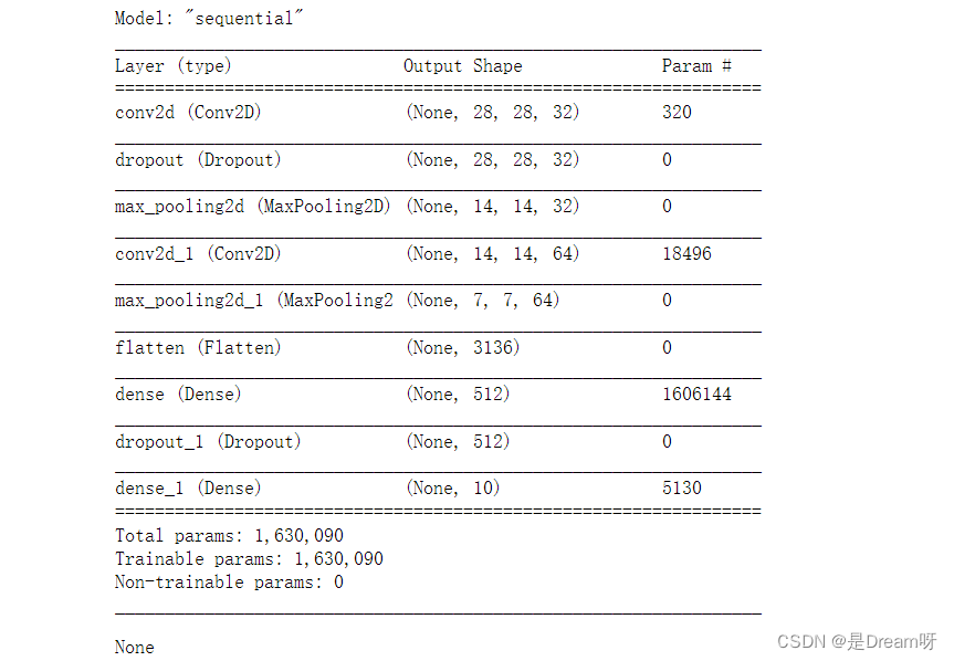
# 展示训练的过程
display(model.summary())
🌟🌟🌟这里是输出的结果:✨✨✨
5.数据增强
在这里我们使用数据增强方法,更好的提高准确率
# 数据增强
datagen = ImageDataGenerator(
        rotation_range=15,
        zoom_range = 0.01,
        width_shift_range=0.1,
        height_shift_range=0.1)
train_gen = datagen.flow(X_train, y_train, batch_size=128)
test_gen = datagen.flow(X_test, y_test, batch_size=128)
6.训练
首先我们批量输入的样本个数,然后经过我们测试分析,此模型训练到30轮之前变化趋于静止,我们可以只进行30个epoch
# 批量输入的样本个数
batch_size = 128
train_steps = X_train.shape[0] // batch_size
valid_steps = X_test.shape[0] // batch_size
# 经过我们测试分析,此模型训练到30轮之前变化趋于静止,我们可以只进行30个epoch
es = tf.keras.callbacks.EarlyStopping(
monitor="val_accuracy",
patience=10,
verbose=1,
mode="max",
restore_best_weights=True)
rp = tf.keras.callbacks.ReduceLROnPlateau(
monitor="val_accuracy",
factor=0.2,
patience=5,
verbose=1,
mode="max",
min_lr=0.00001)
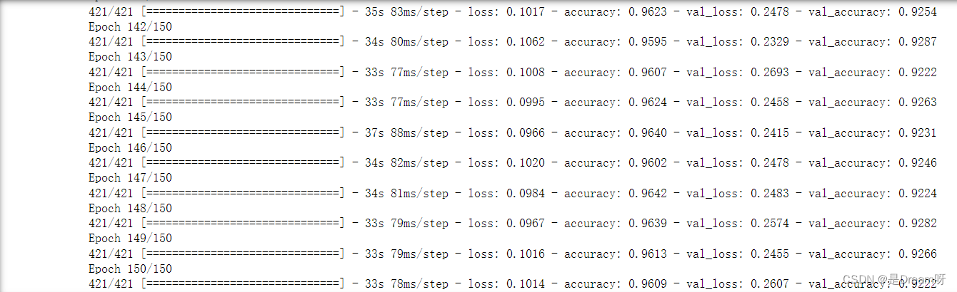
# 训练(训练150个epoch)
history = model.fit(train_gen,
epochs = 150,
steps_per_epoch = train_steps,
validation_data = test_gen,
validation_steps = valid_steps)
🌟🌟🌟这里是输出的结果:✨✨✨
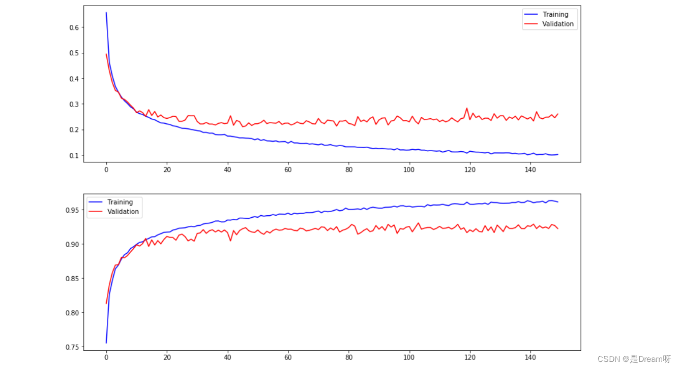
7.画出图像
使用plt模块进行数据可视化处理
fig, ax = plt.subplots(2,1, figsize=(14, 10))
ax[0].plot(history.history['loss'], color='blue', label="Training")
ax[0].plot(history.history['val_loss'], color='red', label="Validation",axes =ax[0])
ax[0].legend(loc='best', shadow=False)

ax[1].plot(history.history['accuracy'], color='blue', label="Training")
ax[1].plot(history.history['val_accuracy'], color='red',label="Validation")
ax[1].legend(loc='best',shadow=False)
plt.show()
🌟🌟🌟这里是输出的结果:✨✨✨
8.输出
最后在测试集上进行模型评估,输出测试集上的预测准确率
score = model.evaluate(X_test, y_test) # 在测试集上进行模型评估
print('测试集预测准确率:', score[1]) # 打印测试集上的预测准确率
🌟🌟🌟 这里是输出的结果:✨✨✨

9.结果
print("The accuracy of the model is %f" %score[1])
The accuracy of the model is 0.931667
三、防止过拟合模型
1.调用库函数
import tensorflow as tf
import matplotlib.pyplot as plt
from sklearn.model_selection import train_test_split
from tensorflow.keras.preprocessing.image import ImageDataGenerator
from tensorflow.keras.layers import Conv2D,MaxPooling2D,BatchNormalization,Flatten,Dense,Dropout
# 指定当前程序使用的 GPU
gpus = tf.config.experimental.list_physical_devices('GPU')
for gpu in gpus:
    tf.config.experimental.set_memory_growth(gpu, True)
2.调用数据集
# 调用数据集
(train_X, train_y),(test_X, test_y) = tf.keras.datasets.fashion_mnist.load_data()
train_X, test_X = train_X / 255.0, test_X / 255.0
train_X = train_X.reshape(-1, 28, 28, 1)
train_y = tf.keras.utils.to_categorical(train_y)
X_train, X_test, y_train, y_test = train_test_split(train_X, train_y, test_size=0.1, random_state=0)
3.选择模型,构建网络
搭建MaxPooling2D层、Conv2D层
# 选择模型,构建网络
model = tf.keras.Sequential()

model.add(Conv2D(32, (3, 3), padding='same', activation=tf.nn.relu,input_shape=(28, 28, 1))), #添加Conv2D层
model.add(Dropout(0.1)),
model.add(MaxPooling2D((2, 2), strides=2)), #添加MaxPooling2D层
model.add(Conv2D(64, (3, 3), padding='same', activation=tf.nn.relu)),#添加Conv2D层
model.add(MaxPooling2D((2, 2), strides=2)),#添加MaxPooling2D层

model.add(Flatten()), #展平
model.add(Dense(512, activation=tf.nn.relu)),
model.add(Dropout(0.1)),
model.add(Dense(10, activation=tf.nn.softmax))
4.编译
使用交叉熵作为loss函数,指明优化器、损失函数及验证过程中的评估指标
# 编译(使用交叉熵作为loss函数)
model.compile(optimizer='adam',  #指定优化器
              loss="categorical_crossentropy",   #指定损失函数
              metrics=['accuracy'])   #指定验证过程中的评估指标
# 展示训练的过程
display(model.summary())
🌟🌟🌟这里是输出的结果:✨✨✨
5.数据增强
在这里我们使用数据增强方法,更好的提高准确率
# 数据增强
datagen = ImageDataGenerator(
        rotation_range=15,
        zoom_range = 0.01,
        width_shift_range=0.1,
        height_shift_range=0.1)
train_gen = datagen.flow(X_train, y_train, batch_size=128)
test_gen = datagen.flow(X_test, y_test, batch_size=128)
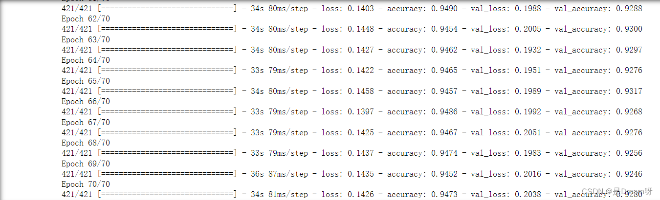
6.训练
首先我们批量输入的样本个数,然后经过我们测试分析,此模型训练到70轮之前变化趋于静止,我们可以只进行70个epoch
# 批量输入的样本个数
batch_size = 128
train_steps = X_train.shape[0] // batch_size
valid_steps = X_test.shape[0] // batch_size

# 经过我们测试分析,此模型训练到70轮之前变化趋于静止,我们可以只进行70个epoch
es = tf.keras.callbacks.EarlyStopping(
        monitor="val_accuracy",
        patience=10,
        verbose=1,
        mode="max",
        restore_best_weights=True)

rp = tf.keras.callbacks.ReduceLROnPlateau(
        monitor="val_accuracy",
        factor=0.2,
        patience=5,
        verbose=1,
        mode="max",
        min_lr=0.00001)

# 训练(训练70个epoch)
history = model.fit(train_gen,
                    epochs = 70,
                    steps_per_epoch = train_steps,
                    validation_data = test_gen,
                    validation_steps = valid_steps,
                   callbacks=[ rp])
🌟🌟🌟这里是输出的结果:✨✨✨
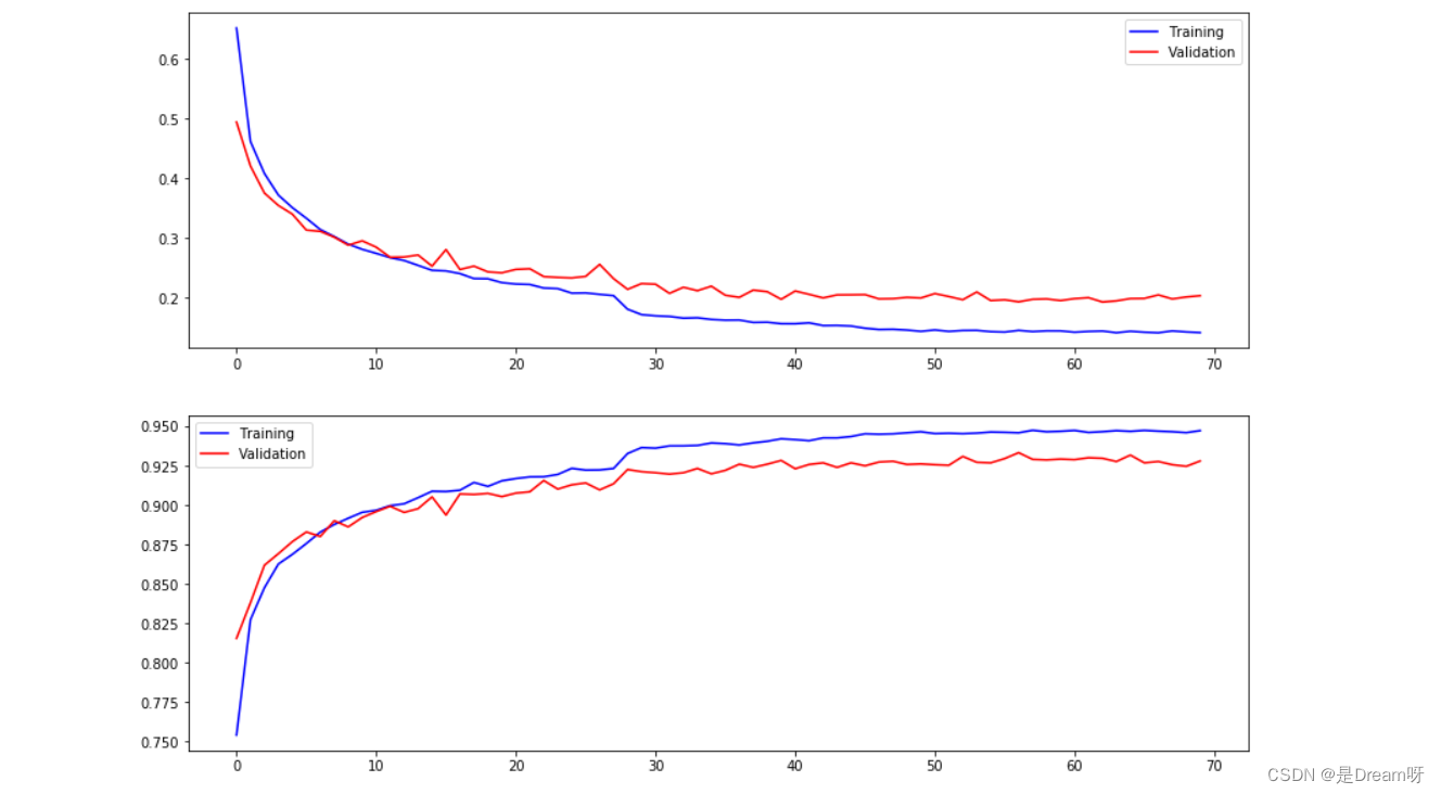
7.画出图像
使用plt模块进行数据可视化处理
fig, ax = plt.subplots(2,1, figsize=(14, 10))
ax[0].plot(history.history['loss'], color='blue', label="Training")
ax[0].plot(history.history['val_loss'], color='red', label="Validation",axes =ax[0])
ax[0].legend(loc='best', shadow=False)

ax[1].plot(history.history['accuracy'], color='blue', label="Training")
ax[1].plot(history.history['val_accuracy'], color='red',label="Validation")
ax[1].legend(loc='best',shadow=False)
plt.show()
🌟🌟🌟这里是输出的结果:✨✨✨
8.输出
最后在测试集上进行模型评估,输出测试集上的预测准确率
score = model.evaluate(X_test, y_test) # 在测试集上进行模型评估
print('测试集预测准确率:', score[1]) # 打印测试集上的预测准确率
🌟🌟🌟这里是输出的结果:✨✨✨

9.结果
print("The accuracy of the model is %f" %score[1])
The accuracy of the model is 0.935833
四、两种模型对比
通过对比前后的两次实验结果,我们发现,没有采用防止过拟合手段,得到的最终准确率为:0.9317;而我们采用防止过拟合的手段,得到的最终准确率为:0.9358,通过对比证明防止过拟手段有效。
五、源码获取
关注此公众号:人生苦短我用Pythons,回复 神经网络实验获取源码,快点击我吧
🌲🌲🌲 好啦,这就是今天要分享给大家的全部内容了,我们下期再见!
❤️❤️❤️如果你喜欢的话,就不要吝惜你的一键三连了~


- 点赞
- 收藏
- 关注作者
评论(0)