ElasticSearch实战指南必知必会：安装中文分词器、ES-Python使用、高级查询实现位置坐标搜索以及打分机制

1.ElasticSearch之-安装中文分词器

elasticsearch 提供了几个内置的分词器：standard analyzer(标准分词器)、simple analyzer(简单分词器)、whitespace analyzer（空格分词器）、language analyzer（语言分词器）

而如果我们不指定分词器类型的话，elasticsearch 默认是使用标准分词器的

我们需要下载中文分词插件，来实现中文分词

• 下载

地址为：

https://github.com/medcl/elasticsearch-analysis-ik

安装方式参照上一篇文章

#采用第二种，url安装
./bin/elasticsearch-plugin install https://github.com/medcl/elasticsearch-analysis-ik/releases/download/v7.4.2/elasticsearch-analysis-ik-7.4.2.zip

2.Elasticsearch之-Python 使用

from elasticsearch import Elasticsearch

obj = Elasticsearch()
#创建索引（Index）
result = obj.indices.create(index='user', body={"userid":'1','username':'lqz'},ignore=400)
#print(result)
#删除索引
#result = obj.indices.delete(index='user', ignore=[400, 404])
#插入数据
#data = {'userid': '1', 'username': 'lqz','password':'123'}
#result = obj.create(index='news', doc_type='politics', id=1, body=data)
#print(result)
#更新数据
'''
不用doc包裹会报错
ActionRequestValidationException[Validation Failed: 1: script or doc is missing
'''
#data ={'doc':{'userid': '1', 'username': 'lqz','password':'123ee','test':'test'}}
#result = obj.update(index='news', doc_type='politics', body=data, id=1)
#print(result)


#删除数据
#result = obj.delete(index='news', doc_type='politics', id=1)

#查询
#查找所有文档
query = {'query': {'match_all': {}}}
#查找名字叫做jack的所有文档
#query = {'query': {'term': {'username': 'lqz'}}}

#查找年龄大于11的所有文档
#query = {'query': {'range': {'age': {'gt': 11}}}}

allDoc = obj.search(index='news', doc_type='politics', body=query)
print(allDoc['hits']['hits'][0]['_source'])

3. Elasticsearch高级之-位置坐标实现附近的人搜索

3.1创建 mapping

PUT test
{
  "mappings": {
    "test":{
      "properties": {
        "location":{
          "type": "geo_point"
        }
      }
    }
  }
}

• 导入数据

POST test/test
{
  "location":{
    "lat":12,
    "lon":24
  }
}

3.2 查询

根据给定两个点组成的矩形，查询矩形内的点

GET test/test/_search
{
  "query": {
    "geo_bounding_box": {
      "location": {
        "top_left": {
          "lat": 28,
          "lon": 10
        },
        "bottom_right": {
          "lat": 10,
          "lon": 30
        }
      }
    }
  }
}

根据给定的多个点组成的多边形，查询范围内的点

GET test/test/_search
{
  "query": {
    "geo_polygon": {
      "location": {
        "points": [
          {
            "lat": 11,
            "lon": 25
          },
          {
            "lat": 13,
            "lon": 25
          },
          {
            "lat": 13,
            "lon": 23
          },
          {
            "lat": 11,
            "lon": 23
          }
        ]
      }
    }
  }
}

查询给定 1000KM 距离范围内的点

GET test/test/_search
{
  "query": {
    "geo_distance": {
      "distance": "1000km",
      "location": {
        "lat": 12,
        "lon": 23
      }
    }
  }
}

查询距离范围区间内的点的数量

GET test/test/_search
{
  "size": 0, 
  "aggs": {
    "myaggs": {
      "geo_distance": {
        "field": "location",
        "origin": {
          "lat": 52.376,
          "lon": 4.894
        },
        "unit": "km", 
        "ranges": [
          {
            "from": 50, 
            "to": 30000
          }
        ]
      }
    }
  }
}

4.Elasticsearch之打分机制

4.1 文档打分的运作机制：TF-IDF

Lucene和es的打分机制是一个公式。将查询作为输入，使用不同的手段来确定每一篇文档的得分，将每一个因素最后通过公式综合起来，返回该文档的最终得分。这个综合考量的过程，就是我们希望相关的文档被优先返回的考量过程。在Lucene和es中这种相关性称为得分。 在开始计算得分之前，es使用了被搜索词条的频率和它有多常见来影响得分，从两个方面理解：

• 一个词条在某篇文档中出现的次数越多，该文档就越相关。
• 一个词条如果在不同的文档中出现的次数越多，它就越不相关！

我们称之为TF-IDF，TF是词频（term frequency），而IDF是逆文档频率（inverse document frequency）。

4.1.2 词频：TF

考虑一篇文档得分的首要方式，是查看一个词条在文档中出现的次数，比如某篇文章围绕es的打分展开的，那么文章中肯定会多次出现相关字眼，当查询时，我们认为该篇文档更符合，所以，这篇文档的得分会更高。 闲的蛋疼的可以Ctrl + f搜一下相关的关键词（es，得分、打分）之类的试试。

4.1.2 逆文档频率：IDF

相对于词频，逆文档频率稍显复杂，如果一个词条在索引中的不同文档中出现的次数越多，那么它就越不重要。 来个例子，示例地址：

The rules-which require employees to work from 9 am to 9 pm
In the weeks that followed the creation of 996.ICU in March
The 996.ICU page was soon blocked on multiple platforms including the messaging tool WeChat and the UC Browser.

假如es索引中，有上述 3 篇文档：

• 词条ICU的文档频率是2，因为它出现在 2 篇文档中，文档的逆源自得分乘以1/DF，DF是该词条的文档频率，这就意味着，由于ICU词条拥有更高的文档频率，所以，它的权重会降低。
• 词条the的文档频率是3，它在 3 篇文档中都出现了，注意：尽管the在后两篇文档出都出现两次，但是它的词频是还是3，因为，逆文档词频只检查词条是否出现在某篇文档中，而不检查它在这篇文档中出现了多少次，那是词频该干的事儿。

逆文档词频是一个重要的因素，用来平衡词条的词频。比如我们搜索the 996.ICU。单词the几乎出现在所有的文档中（中文中比如的），如果这个鬼东西要不被均衡一下，那么the的频率将完全淹没996.ICU。所以，逆文档词频就有效的均衡了the这个常见词的相关性影响。以达到实际的相关性得分将会对查询的词条有一个更准确地描述。 当词频和逆文档词频计算完成。就可以使用TF-IDF公式来计算文档的得分了。

4.2 Lucene 评分公式

之前的讨论Lucene默认评分公式被称为TF-IDF，一个基于词频和逆文档词频的公式。Lucene实用评分公式如下：

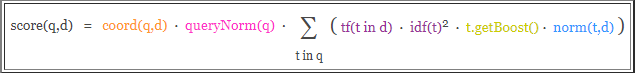
你以为我会着重介绍这个该死的公式？！ 我只能说，词条的词频越高，得分越高；相似地，索引中词条越罕见，逆文档频率越高，其中再加商调和因子和查询标准化，调和因子考虑了搜索过多少文档以及发现了多少词条；查询标准化，是试图让不同的查询结果具有可比性，这显然… 很困难。 我们称这种默认的打分方法是TF-IDF和向量空间模型（vector space model）的结合。

4.3 其他的打分方法

除了TF-IDF结合向量空间模型的实用评分模式，是es和Lucene最为主流的评分机制，但这并不是唯一的，除了TF-IDF这种实用模型之外，其他的模型包括：

• Okapi BM25。
• 随机性分歧（Divergence from randomness），即 DFR 相似度。
• LM Dirichlet 相似度。
• LM Jelinek Mercer 相似度。

这里简要的介绍BM25几种主要设置，即k1、b和discount_overlaps：

• k1 和 b 是数值的设置，用于调整得分是如何计算的。
• k1 控制对于得分而言词频（TF）的重要性。
• b 是介于0 ~ 1之间的数值，它控制了文档篇幅对于得分的影响程度。
• 默认情况下，k1设置为1.2，而b则被设置为0.75
• discount_overlaps的设置用于告诉es，在某个字段中，多少个分词出现在同一位置，是否应该影响长度的标准化，默认值是true。

4.4 配置打分模型

4.4.1 简要配置 BM25 打分模型

BM25（是不是跟 pm2.5 好像！！！）是一种基于概率的打分框架。我们来简要的配置一下：

PUT w2
{
  "mappings": {
    "doc": {
      "properties": {
        "title": {
          "type": "text",
          "similarity": "BM25"
        }
      }
    }
  }
}

PUT w2/doc/1
{
  "title":"The rules-which require employees to work from 9 am to 9 pm"
}

PUT w2/doc/2
{
  "title":"In the weeks that followed the creation of 996.ICU in March"
}

PUT w2/doc/3
{
  "title":"The 996.ICU page was soon blocked on multiple platforms including the messaging tool WeChat and the UC Browser."
}

GET w2/doc/_search
{
  "query": {
    "match": {
      "title": "the 996"
    }
  }
}

上例是通过similarity参数来指定打分模型。至于查询，还是当数据量比较大的时候，多试几次，比较容易发现不同之处。

4.4.2 为 BM25 配置高级的 settings

PUT w3
{
  "settings": {
    "index": {
      "analysis": {
        "analyzer":"ik_smart"
      }
    },
    "similarity": {
      "my_custom_similarity": {
        "type": "BM25",
        "k1": 1.2,
        "b": 0.75,
        "discount_overlaps": false
      }
    }
  },
  "mappings": {
    "doc": {
      "properties": {
        "title": {
          "type": "text",
          "similarity":"my_custom_similarity"
        }
      }
    }
  }
}

PUT w3/doc/1
{
  "title":"The rules-which require employees to work from 9 am to 9 pm"
}

PUT w3/doc/2
{
  "title":"In the weeks that followed the creation of 996.ICU in March"
}

PUT w3/doc/3
{
  "title":"The 996.ICU page was soon blocked on multiple platforms including the messaging tool WeChat and the UC Browser."
}

GET w3/doc/_search
{
  "query": {
    "match": {
      "title": "the 996"
    }
  }
}

4.4.3 配置全局打分模型

如果我们要使用某种特定的打分模型，并且希望应用到全局，那么就在elasticsearch.yml配置文件中加入：

index.similarity.default.type: BM25

4.5. boosting

boosting是一个用来修改文档相关性的程序。boosting有两种类型：

• 索引的时候，比如我们在定义 mappings 的时候。
• 查询一篇文档的时候。

以上两种方式都可以提升一个篇文档的得分。需要注意的是：在索引期间修改的文档 boosting 是存储在索引中的，要想修改 boosting 必须重新索引该篇文档。

4.5.1 索引期间的 boosting

啥也不说了，都在酒里！上代码：

PUT w4
{
  "mappings": {
    "doc": {
      "properties": {
        "name": {
          "boost": 2.0,
          "type": "text"
        },
        "age": {
          "type": "long"
        }
      }
    }
  }
}

一劳永逸是没错，但一般不推荐这么玩。

原因之一是因为一旦映射建立完成，那么所有name字段都会自动拥有一个boost值。要想修改这个值，那就必须重新索引文档。 另一个原因是，boost值是以降低精度的数值存储在Lucene内部的索引结构中。只有一个字节用于存储浮点型数值（存不下就损失精度了），所以，计算文档的最终得分时可能会损失精度。 最后，boost是应用与词条的。因此，再被boost的字段中如果匹配上了多个词条，就意味着计算多次的boost，这将会进一步增加字段的权重，可能会影响最终的文档得分。 现在我们再来介绍另一种方式。

4.5.2 查询期间的 boosting

在es中，几乎所有的查询类型都支持boost，正如你想象的那些match、multi_match等等。 来个示例，在查询期间，使用 match 查询进行boosting：

PUT w5
{
  "mappings":{
    "doc":{
      "properties": {
        "title": {
          "type": "text",
          "analyzer": "ik_max_word"
        },
        "content": {
          "type": "text",
          "analyzer": "ik_max_word"
        }
      }
    }
  }
}

PUT w5/doc/1
{
  "title":"Lucene is cool",
  "content": "Lucene is cool"
}

PUT w5/doc/2
{
  "title":"Elasticsearch builds on top of lucene",
  "content":"Elasticsearch builds on top of lucene"
}

PUT w5/doc/3
{
  "title":"Elasticsearch rocks",
  "content":"Elasticsearch rocks"
}

来查询：

GET w5/doc/_search
{
  "query": {
    "bool": {
      "should": [
        {
          "match": {
            "title":{
              "query": "elasticserach rocks",
              "boost": 2.5
            }
          }
        },
        {
          "match": {
            "content": "elasticserach rocks"
          }
        }
      ]
    }
  }
}

就对于最终得分而言，content字段，加了boost的title查询更有影响力。也只有在bool查询中，boost更有意义。

4.5.3 跨越多个字段的查询

boost也可以用于multi_match查询。

GET w5/doc/_search
{
  "query": {
    "multi_match": {
      "query": "elasticserach rocks",
      "fields": ["title", "content"],
      "boost": 2.5
    }
  }
}

除此之外，我们还可以使用特殊的语法，只为特定的字段指定一个boost。通过在字段名称后添加一个^符号和boost的值。告诉 es 只需对那个字段进行boost：

GET w5/doc/_search
{
  "query": {
    "multi_match": {
      "query": "elasticserach rocks",
      "fields": ["title^3", "content"]
    }
  }
}

上例中，title字段被boost了 3 倍。 需要注意的是：在使用boost的时候，无论是字段或者词条，都是按照相对值来boost的，而不是乘以乘数。如果对于所有的待搜索词条boost了同样的值，那么就好像没有boost一样（废话，就像大家都同时长高一米似的）！因为 Lucene 会标准化boost的值。如果boost一个字段4倍，不是意味着该字段的得分就是乘以4的结果。所以，如果你的得分不是按照严格的乘法结果，也不要担心。

5.带你理解文档是如何评分的

一切都不是你想的那样！是的，在es中，一个文档要比另一个文档更符合某个查询很可能跟我们想象的不太一样！ 这一小节，我们来研究下es和Lucene内部使用了怎样的公式来计算得分。 我们通过explain=true来告诉es，你要给洒家解释一下为什么这个得分是这样的？！背后到底以有什么 py 交易！ 比如我们来查询：

GET py1/doc/_search
{
  "query": {
    "match": {
      "title": "北京"
    }
  },
  "explain": true,
  "_source": "title", 
  "size": 1
}

由于结果太长，我们这里对结果进行了过滤（"size": 1返回一篇文档），只查看指定的字段（"_source": "title"只返回title字段）。 看结果：

{
  "took" : 1,
  "timed_out" : false,
  "_shards" : {
    "total" : 5,
    "successful" : 5,
    "skipped" : 0,
    "failed" : 0
  },
  "hits" : {
    "total" : 24,
    "max_score" : 4.9223156,
    "hits" : [
      {
        "_shard" : "[py1][1]",
        "_node" : "NRwiP9PLRFCTJA7w3H9eqA",
        "_index" : "py1",
        "_type" : "doc",
        "_id" : "NIjS1mkBuoj17MYtV-dX",
        "_score" : 4.9223156,
        "_source" : {
          "title" : "大写的尴尬 插混为啥在北京不受待见？"
        },
        "_explanation" : {
          "value" : 4.9223156,
          "description" : "weight(title:北京 in 36) [PerFieldSimilarity], result of:",
          "details" : [
            {
              "value" : 4.9223156,
              "description" : "score(doc=36,freq=1.0 = termFreq=1.0\n), product of:",
              "details" : [
                {
                  "value" : 4.562031,
                  "description" : "idf, computed as log(1 + (docCount - docFreq + 0.5) / (docFreq + 0.5)) from:",
                  "details" : [
                    {
                      "value" : 4.0,
                      "description" : "docFreq",
                      "details" : [ ]
                    },
                    {
                      "value" : 430.0,
                      "description" : "docCount",
                      "details" : [ ]
                    }
                  ]
                },
                {
                  "value" : 1.0789746,
                  "description" : "tfNorm, computed as (freq * (k1 + 1)) / (freq + k1 * (1 - b + b * fieldLength / avgFieldLength)) from:",
                  "details" : [
                    {
                      "value" : 1.0,
                      "description" : "termFreq=1.0",
                      "details" : [ ]
                    },
                    {
                      "value" : 1.2,
                      "description" : "parameter k1",
                      "details" : [ ]
                    },
                    {
                      "value" : 0.75,
                      "description" : "parameter b",
                      "details" : [ ]
                    },
                    {
                      "value" : 12.1790695,
                      "description" : "avgFieldLength",
                      "details" : [ ]
                    },
                    {
                      "value" : 10.0,
                      "description" : "fieldLength",
                      "details" : [ ]
                    }
                  ]
                }
              ]
            }
          ]
        }
      }
    ]
  }
}

在新增的_explanation字段中，可以看到value值是4.9223156，那么是怎么算出来的呢？ 来分析，分词北京在描述字段（title）出现了1次，所以TF的综合得分经过"description" : "tfNorm, computed as (freq * (k1 + 1)) / (freq + k1 * (1 - b + b * fieldLength / avgFieldLength)) from:"计算，得分是1.0789746。 那么逆文档词频呢？根据"description" : "idf, computed as log(1 + (docCount - docFreq + 0.5) / (docFreq + 0.5)) from:"计算得分是4.562031。 所以最终得分是：

1.0789746 * 4.562031 = 4.9223155734126

结果在四舍五入后就是4.9223156。 需要注意的是，explain的特性会给es带来额外的性能开销。所以，除了在调试时可以使用，生产环境下，应避免使用explain。

更多优质内容请关注公号：汀丶人工智能；会提供一些相关的资源和优质文章，免费获取阅读。