【数据分析】——Numpy:基本操作快速入门

目录

Numpy是一个用python实现的科学计算的扩展程序库,包括:
- 1、一个强大的N维数组对象Array;
- 2、比较成熟的(广播)函数库;
- 3、用于整合C/C++和Fortran代码的工具包;
- 4、实用的线性代数、傅里叶变换和随机数生成函数。numpy和稀疏矩阵运算包scipy配合使用更加方便。
1.Numpy基本操作
1.1 列表转为矩阵
import numpy as np
array = np.array([
    [1,3,5],
    [4,6,9]
])

print(array)
[[1 3 5] [4 6 9]]
1.2 维度
print('number of dim:', array.ndim)number of dim: 21.3 行数和列数()
print('shape:',array.shape)shape: (2, 3)1.4 元素个数
print('size:',array.size)size: 6
2.Numpy创建array
2.1 一维array创建
import numpy as np
# 一维array
a = np.array([2,23,4], dtype=np.int32) # np.int默认为int32
print(a)
print(a.dtype)
[ 2 23 4]
int322.2 多维array创建
# 多维array
a = np.array([[2,3,4],
              [3,4,5]])
print(a) # 生成2行3列的矩阵
2.3 创建全零数组
a = np.zeros((3,4))
print(a) # 生成3行4列的全零矩阵
[[0. 0. 0. 0.]
[0. 0. 0. 0.]
[0. 0. 0. 0.]]2.4 创建全1数据
# 创建全一数据,同时指定数据类型
a = np.ones((3,4),dtype=np.int)
print(a)
[[1 1 1 1]
[1 1 1 1]
[1 1 1 1]]2.5 创建全空数组
# 创建全空数组,其实每个值都是接近于零的数
a = np.empty((3,4))
print(a)
[[0. 0. 0. 0.]
[0. 0. 0. 0.]
[0. 0. 0. 0.]]2.6 创建连续数组
# 创建连续数组
a = np.arange(10,21,2) # 10-20的数据,步长为2
print(a)
[10 12 14 16 18 20]2.7 reshape操作
# 使用reshape改变上述数据的形状
b = a.reshape((2,3))
print(b)
[[10 12 14]
[16 18 20]]2.8 创建连续型数据
# 创建线段型数据
a = np.linspace(1,10,20) # 开始端1,结束端10,且分割成20个数据,生成线段
print(a)
[ 1. 1.47368421 1.94736842 2.42105263 2.89473684 3.36842105
3.84210526 4.31578947 4.78947368 5.26315789 5.73684211 6.21052632
6.68421053 7.15789474 7.63157895 8.10526316 8.57894737 9.05263158
9.52631579 10. ]2.9 linspace的reshape操作
# 同时也可以reshape
b = a.reshape((5,4))
print(b)
[[ 1. 1.47368421 1.94736842 2.42105263]
[ 2.89473684 3.36842105 3.84210526 4.31578947]
[ 4.78947368 5.26315789 5.73684211 6.21052632]
[ 6.68421053 7.15789474 7.63157895 8.10526316]
[ 8.57894737 9.05263158 9.52631579 10. ]]3.Numpy基本运算
3.1 一维矩阵运算
import numpy as np
# 一维矩阵运算
a = np.array([10,20,30,40])
b = np.arange(4)
print(a,b)
[10 20 30 40] [0 1 2 3]c = a - b
print(c)[10 19 28 37]print(a*b) # 若用a.dot(b),则为各维之和[ 0 20 60 120]# 在Numpy中,想要求出矩阵中各个元素的乘方需要依赖双星符号 **,以二次方举例,即:
c = b**2
print(c)[0 1 4 9]# Numpy中具有很多的数学函数工具
c = np.sin(a)
print(c)[-0.54402111 0.91294525 -0.98803162 0.74511316]print(b<2)[ True True False False]a = np.array([1,1,4,3])
b = np.arange(4)
print(a==b)[False True False True]3.2 多维矩阵运算
a = np.array([[1,1],[0,1]])
b = np.arange(4).reshape((2,2))
print(a)
[[1 1]
[0 1]]
print(b)[[0 1]
[2 3]]# 多维度矩阵乘法
# 第一种乘法方式:
c = a.dot(b)
print(c)[[2 4]
[2 3]]
# 第二种乘法:
c = np.dot(a,b)
print(c)
[[2 4]
[2 3]]
3.825517216750851
print(np.min(a))0.09623355767721398
print(np.max(a))0.7420428188342583
print("a=",a)a= [[0.48634962 0.74204282 0.09623356 0.69074812]
[0.60218881 0.52734181 0.41434585 0.26626662]]
如果你需要对行或者列进行查找运算,
就需要在上述代码中为 axis 进行赋值。
当axis的值为0的时候,将会以列作为查找单元,
当axis的值为1的时候,将会以行作为查找单元。
print("sum=",np.sum(a,axis=1))sum= [2.01537412 1.8101431 ]
print("min=",np.min(a,axis=0))min= [0.48634962 0.52734181 0.09623356 0.26626662]
print("max=",np.max(a,axis=1))max= [0.74204282 0.60218881]3.3 基本计算
import numpy as np
A = np.arange(2,14).reshape((3,4))
print(A)
[[ 2 3 4 5]
[ 6 7 8 9]
[10 11 12 13]]
# 最小元素索引
print(np.argmin(A)) # 0
0
# 最大元素索引
print(np.argmax(A)) # 11
11
# 求整个矩阵的均值
print(np.mean(A)) # 7.5
7.5
print(np.average(A)) # 7.57.5
print(A.mean()) # 7.57.5
# 中位数
print(np.median(A)) # 7.5
7.5
# 累加
print(np.cumsum(A))
[ 2 5 9 14 20 27 35 44 54 65 77 90]
# 累差运算
B = np.array([[3,5,9],
              [4,8,10]])
print(np.diff(B))
[[2 4]
[4 2]]
C = np.array([[0,5,9],
              [4,0,10]])
print(np.nonzero(B))
print(np.nonzero(C))
(array([0, 0, 0, 1, 1, 1], dtype=int64), array([0, 1, 2, 0, 1, 2], dtype=int64))
(array([0, 0, 1, 1], dtype=int64), array([1, 2, 0, 2], dtype=int64))
# 仿照列表排序
A = np.arange(14,2,-1).reshape((3,4)) # -1表示反向递减一个步长
print(A)
[[14 13 12 11]
[10 9 8 7]
[ 6 5 4 3]]
print(np.sort(A))[[11 12 13 14]
[ 7 8 9 10]
[ 3 4 5 6]]
# 矩阵转置
print(np.transpose(A))
[[14 10 6]
[13 9 5]
[12 8 4]
[11 7 3]]
print(A.T)[[14 10 6]
[13 9 5]
[12 8 4]
[11 7 3]]
print(A)[[14 13 12 11]
[10 9 8 7]
[ 6 5 4 3]]
print(np.clip(A,5,9))[[9 9 9 9]
[9 9 8 7]
[6 5 5 5]]
clip(Array,Array_min,Array_max)
将Array_min<X<Array_max X表示矩阵A中的数,如果满足上述关系,则原数不变。
否则,如果X<Array_min,则将矩阵中X变为Array_min;
如果X>Array_max,则将矩阵中X变为Array_max.
4.Numpy索引与切片
import numpy as np
A = np.arange(3,15)
print(A)
[ 3 4 5 6 7 8 9 10 11 12 13 14]
print(A[3])6
B = A.reshape(3,4)
print(B)
[[ 3 4 5 6]
[ 7 8 9 10]
[11 12 13 14]]
print(B[2])[11 12 13 14]
print(B[0][2])5
print(B[0,2])5
# list切片操作
print(B[1,1:3]) # [8 9] 1:3表示1-2不包含3
[8 9]
for row in B:
    print(row)
[3 4 5 6]
[ 7 8 9 10]
[11 12 13 14]
# 如果要打印列,则进行转置即可
for column in B.T:
    print(column)
[ 3 7 11]
[ 4 8 12]
[ 5 9 13]
[ 6 10 14]
# 多维转一维
A = np.arange(3,15).reshape((3,4))
# print(A)
print(A.flatten())
# flat是一个迭代器,本身是一个object属性
[ 3 4 5 6 7 8 9 10 11 12 13 14]
for item in A.flat:
    print(item)
3
4
5
6
7
8
9
10
11
12
13
14
我们一起来来总结一下,看下面切片取值方式(对应颜色是取出来的结果):
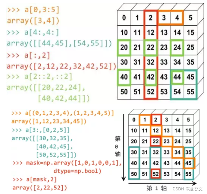
![]()
5.Numpy array合并
5.1 数组合并
import numpy as np
A = np.array([1,1,1])
B = np.array([2,2,2])
print(np.vstack((A,B)))
# vertical stack 上下合并,对括号的两个整体操作。
[[1 1 1]
[2 2 2]]
C = np.vstack((A,B))
print(C)
[[1 1 1]
[2 2 2]]
print(A.shape,B.shape,C.shape)# 从shape中看出A,B均为拥有3项的数组(数列)(3,) (3,) (2, 3)
# horizontal stack左右合并
D = np.hstack((A,B))
print(D)
[1 1 1 2 2 2]
(3,) (3,) (6,)
5.2 数组转置为矩阵
print(A[np.newaxis,:]) # [1 1 1]变为[[1 1 1]][[1 1 1]]
print(A[np.newaxis,:].shape) # (3,)变为(1, 3)(1, 3)
print(A[:,np.newaxis])[[1]
[1]
[1]]
5.3 多个矩阵合并
# concatenate的第一个例子
print("------------")
print(A[:,np.newaxis].shape) # (3,1)
------------
(3, 1)
A = A[:,np.newaxis] # 数组转为矩阵
B = B[:,np.newaxis] # 数组转为矩阵print(A)[[1]
[1]
[1]]
print(B)[[2]
[2]
[2]]
[[1]
 [1]
 [1]
 [2]
 [2]
 [2]
 [2]
 [2]
 [2]
 [1]
 [1]
 [1]]
# axis=1横向合并
C = np.concatenate((A,B),axis=1)
print(C)
[[1 2]
[1 2]
[1 2]]
5.4 合并例子2
# concatenate的第二个例子
print("-------------")
a = np.arange(8).reshape(2,4)
b = np.arange(8).reshape(2,4)
print(a)
print(b)
print("-------------")
-------------
[[0 1 2 3]
[4 5 6 7]]
[[0 1 2 3]
[4 5 6 7]]
-------------
# axis=0多个矩阵纵向合并
c = np.concatenate((a,b),axis=0)
print(c)
[[0 1 2 3]
[4 5 6 7]
[0 1 2 3]
[4 5 6 7]]
# axis=1多个矩阵横向合并
c = np.concatenate((a,b),axis=1)
print(c)
[[0 1 2 3 0 1 2 3]
[4 5 6 7 4 5 6 7]]6.Numpy array分割
6.1 构造3行4列矩阵
import numpy as np
A = np.arange(12).reshape((3,4))
print(A)
[[ 0 1 2 3]
[ 4 5 6 7]
[ 8 9 10 11]]
6.2 等量分割
# 等量分割
# 纵向分割同横向合并的axis
print(np.split(A, 2, axis=1))
[array([[0, 1],
[4, 5],
[8, 9]]), array([[ 2, 3],
[ 6, 7],
[10, 11]])]
# 横向分割同纵向合并的axis
print(np.split(A,3,axis=0))
[array([[0, 1, 2, 3]]), array([[4, 5, 6, 7]]), array([[ 8, 9, 10, 11]])]
6.3 不等量分割
print(np.array_split(A,3,axis=1))[array([[0, 1],
[4, 5],
[8, 9]]), array([[ 2],
[ 6],
[10]]), array([[ 3],
[ 7],
[11]])]
6.4 其他的分割方式
# 横向分割
print(np.vsplit(A,3)) # 等价于print(np.split(A,3,axis=0))
[array([[0, 1, 2, 3]]), array([[4, 5, 6, 7]]), array([[ 8, 9, 10, 11]])]
# 纵向分割
print(np.hsplit(A,2)) # 等价于print(np.split(A,2,axis=1))
[array([[0, 1],
[4, 5],
[8, 9]]), array([[ 2, 3],
[ 6, 7],
[10, 11]])]7.Numpy copy与 =
7.1 =赋值方式会带有关联性
import numpy as np
# `=`赋值方式会带有关联性
a = np.arange(4)
print(a) # [0 1 2 3]
[0 1 2 3]
b = a
c = a
d = b
a[0] = 11
print(a) # [11  1  2  3]
[11 1 2 3]
print(b) # [11 1 2 3][11 1 2 3]
print(c) # [11 1 2 3][11 1 2 3]
print(d) # [11 1 2 3][11 1 2 3]
print(b is a) # TrueTrue
print(c is a) # TrueTrue
print(d is a) # TrueTrue
d[1:3] = [22,33]
print(a) # [11 22 33  3]
[11 22 33 3]
print(b) # [11 22 33 3][11 22 33 3]
print(c) # [11 22 33 3][11 22 33 3]
7.2 copy()赋值方式没有关联性
a = np.arange(4)
print(a) # [0 1 2 3]
[0 1 2 3]
b =a.copy() # deep copy
print(b) # [0 1 2 3]
[0 1 2 3]
a[3] = 44
print(a) # [ 0 1 2 44]
print(b) # [0 1 2 3]
# 此时a与b已经没有关联[ 0 1 2 44]
[0 1 2 3]8.广播机制
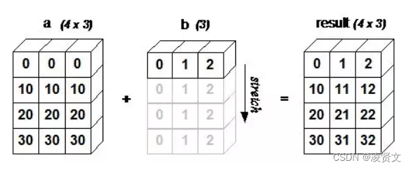
numpy数组间的基础运算是一对一,也就是a.shape==b.shape,但是当两者不一样的时候,就会自动触发广播机制,如下例子:
from numpy import array
a = array([[ 0, 0, 0],
           [10,10,10],
           [20,20,20],
           [30,30,30]])
b = array([0,1,2])
print(a+b)
[[ 0 1 2]
[10 11 12]
[20 21 22]
[30 31 32]]
为什么是这个样子?
这里以tile模拟上述操作,来回到a.shape==b.shape情况!
# 对[0,1,2]行重复3次,列重复1次
b = np.tile([0,1,2],(4,1))
print(a+b)
[[ 0 1 2]
[10 11 12]
[20 21 22]
[30 31 32]]
到这里,我们来给出一张图
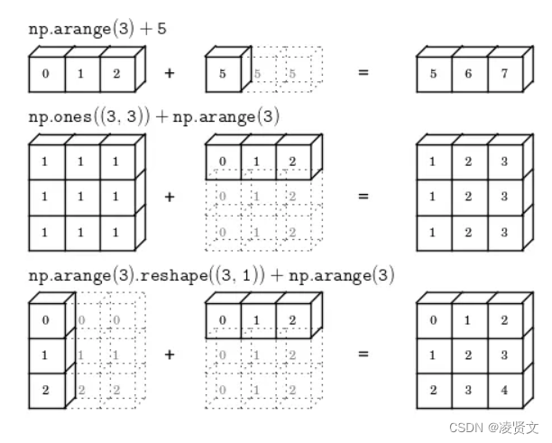
是不是任何情况都可以呢?
当然不是,只有当两个数组的trailing dimensions compatible时才会触发广播,否则报错ValueError: frames are not aligned exception。
上面表达意思是尾部维度必须兼容!
9.常用函数
9.1 np.bincount()
array([1, 2, 1, 2, 1], dtype=int64)统计索引出现次数:索引0出现1次,1出现2次,2出现1次,3出现2次,4出现1次
因此通过bincount计算出索引出现次数如下:
上面怎么得到的?
对于bincount计算吗,bin的数量比x中最大数多1,例如x最大为4,那么bin数量为5(index从0到4),也就会bincount输出的一维数组为5个数,bincount中的数又代表什么?代表的是它的索引值在x中出现的次数!
还是以上述x为例子,当我们设置weights参数时候,结果又是什么?
这里假定:
w = np.array([0.3,0.5,0.7,0.6,0.1,-0.9,1])那么设置这个w权重后,结果为多少?
np.bincount(x,weights=w)array([ 0.1, -0.6, 0.5, 1.3, 1. ])怎么计算的?
先对x与w抽取出来:
x ---> [1, 2, 3, 3, 0, 1, 4]
w ---> [0.3,0.5,0.7,0.6,0.1,-0.9,1] 索引 0 出现在x中index=4位置,那么在w中访问index=4的位置即可,w[4]=0.1
索引 1 出现在x中index=0与index=5位置,那么在w中访问index=0与index=5的位置即可,然后将两这个加和,计算得:w[0]+w[5]=-0.6 其余的按照上面的方法即可!
bincount的另外一个参数为minlength,这个参数简单,可以这么理解,当所给的bin数量多于实际从x中得到的bin数量后,后面没有访问到的设置为0即可。
还是上述x为例:
这里我们直接设置minlength=7参数,并输出!
np.bincount(x,weights=w,minlength=7)array([ 0.1, -0.6, 0.5, 1.3, 1. , 0. , 0. ])与上面相比多了两个0,这两个怎么会多?
上面知道,这个bin数量为5,index从0到4,那么当minlength为7的时候,也就是总长为7,index从0到6,多了后面两位,直接补位为0即可!
9.2 np.argmax()
函数原型为:numpy.argmax(a, axis=None, out=None).
函数表示返回沿轴axis最大值的索引。
x = [[1,3,3],
     [7,5,2]]
print(np.argmax(x))
3
对于这个例子我们知道,7最大,索引位置为3(这个索引按照递增顺序)!
axis属性
axis=0表示按列操作,也就是对比当前列,找出最大值的索引!
x = [[1,3,3],
     [7,5,2]]
print(np.argmax(x,axis=0))
[1 1 0]
axis=1表示按行操作,也就是对比当前行,找出最大值的索引!
x = [[1,3,3],
     [7,5,2]]
print(np.argmax(x,axis=0))
[1 1 0]
那如果碰到重复最大元素?
返回第一个最大值索引即可!
例如:
x = np.array([1, 3, 2, 3, 0, 1, 0])
print(x.argmax())
1
9.3 上述合并实例
这里来融合上述两个函数,举个例子:
x = np.array([1, 2, 3, 3, 0, 1, 4])
print(np.argmax(np.bincount(x)))
1
最终结果为1,为什么?
首先通过np.bincount(x)得到的结果是:[1 2 1 2 1],再根据最后的遇到重复最大值项,则返回第一个最大值的index即可!2的index为1,所以返回1。
9.4 求取精度
np.around([-0.6,1.2798,2.357,9.67,13], decimals=0)#取指定位置的精度array([-1., 1., 2., 10., 13.])看到没,负数进位取绝对值大的!
np.around([1.2798,2.357,9.67,13], decimals=1)array([ 1.3, 2.4, 9.7, 13. ])np.around([1.2798,2.357,9.67,13], decimals=2)array([ 1.28, 2.36, 9.67, 13. ])从上面可以看出,decimals表示指定保留有效数的位数,当超过5就会进位(此时包含5)!
但是,如果这个参数设置为负数,又表示什么?
np.around([1,2,5,6,56], decimals=-1)array([ 0, 0, 0, 10, 60])发现没,当超过5时候(不包含5),才会进位!-1表示看一位数进位即可,那么如果改为-2呢,那就得看两位!
np.around([1,2,5,50,56,190], decimals=-2)array([ 0, 0, 0, 0, 100, 200])看到没,必须看两位,超过50才会进位,190的话,就看后面两位,后两位90超过50,进位,那么为200!
计算沿指定轴第N维的离散差值
x = np.arange(1 , 16).reshape((3 , 5))
print(x)
[[ 1 2 3 4 5]
[ 6 7 8 9 10]
[11 12 13 14 15]]
np.diff(x,axis=1) #默认axis=1array([[1, 1, 1, 1],
[1, 1, 1, 1],
[1, 1, 1, 1]])
np.diff(x,axis=0) array([[5, 5, 5, 5, 5],
[5, 5, 5, 5, 5]])取整
np.floor([-0.6,-1.4,-0.1,-1.8,0,1.4,1.7])array([-1., -2., -1., -2., 0., 1., 1.])看到没,负数取整,跟上述的around一样,是向左!
取上限
np.ceil([1.2,1.5,1.8,2.1,2.0,-0.5,-0.6,-0.3])array([ 2., 2., 2., 3., 2., -0., -0., -0.])取上限!找这个小数的最大整数即可!
查找
利用np.where实现小于0的值用0填充吗,大于0的数不变!
[[ 1  0]
 [ 2 -2]
 [-2  1]]
np.where(x>0,x,0)array([[1, 0],
[2, 0],
[0, 1]])
部分参考光城同学。

- 点赞
- 收藏
- 关注作者
评论(0)