@toc

1、概述

  LSTM网络是序列模型，一般比较适合处理序列问题。这里把它用于手写数字图片的分类，其实就相当于把图片看作序列。

  一张MNIST数据集的图片是 $28\times 28$的大小，我们可以把每一行看作是一个序列输入，那么一张图片就是28行，序列长度为28；每一行有28个数据，每个序列输入28个值。

  这里我们可以将LSTM和CNN的代码结果进行对比。

2、LSTM实现

import tensorflow as tf
from tensorflow.keras.models import Sequential
from tensorflow.keras.layers import Dense
from tensorflow.keras.layers import LSTM,Dropout
from tensorflow.keras.optimizers import Adam
import matplotlib.pyplot as plt

2.1 载入数据集

# 载入数据集
mnist = tf.keras.datasets.mnist
# 载入数据，数据载入的时候就已经划分好训练集和测试集
# 训练集数据x_train的数据形状为（60000，28，28）
# 训练集标签y_train的数据形状为（60000）
# 测试集数据x_test的数据形状为（10000，28，28）
# 测试集标签y_test的数据形状为（10000）
(x_train, y_train), (x_test, y_test) = mnist.load_data()
# 对训练集和测试集的数据进行归一化处理，有助于提升模型训练速度
x_train, x_test = x_train / 255.0, x_test / 255.0
# 把训练集和测试集的标签转为独热编码
y_train = tf.keras.utils.to_categorical(y_train,num_classes=10)
y_test = tf.keras.utils.to_categorical(y_test,num_classes=10)

# 数据大小-一行有28个像素
input_size = 28
# 序列长度-一共有28行
time_steps = 28
# 隐藏层memory block个数
cell_size = 50 

2.2 创建模型

# 创建模型
# 循环神经网络的数据输入必须是3维数据
# 数据格式为(数据数量，序列长度，数据大小)
# 载入的mnist数据的格式刚好符合要求
# 注意这里的input_shape设置模型数据输入时不需要设置数据的数量
model = Sequential([
    LSTM(units=cell_size,input_shape=(time_steps,input_size),return_sequences=True),
    Dropout(0.2),
    LSTM(cell_size),
    Dropout(0.2),
    # 50个memory block输出的50个值跟输出层10个神经元全连接
    Dense(10,activation=tf.keras.activations.softmax)
])

2.3 定义优化器

adam = Adam(lr=1e-3)

2.4 编译模型

model.compile(optimizer=adam,loss='categorical_crossentropy',metrics=['accuracy'])

2.5 训练模型

history=model.fit(x_train,y_train,batch_size=64,epochs=10,validation_data=(x_test,y_test))

2.6 打印模型摘要

model.summary()

2.7 绘制acc和loss曲线

loss=history.history['loss']
val_loss=history.history['val_loss']

accuracy=history.history['accuracy']
val_accuracy=history.history['val_accuracy']

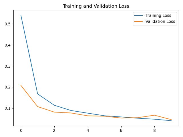
# 绘制loss曲线
plt.plot(loss, label='Training Loss')
plt.plot(val_loss, label='Validation Loss')
plt.title('Training and Validation Loss')
plt.legend()
plt.show()

# 绘制acc曲线
plt.plot(accuracy, label='Training accuracy')
plt.plot(val_accuracy, label='Validation accuracy')
plt.title('Training and Validation Loss')
plt.legend()
plt.show()

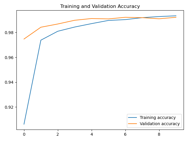
   LSTM应用于MNIST数据识别也可以得到不错的结果，但当然没有卷积神经网络得到的结果好。

3、CNN实现

import tensorflow as tf
from tensorflow.keras.models import Sequential
from tensorflow.keras.layers import Dense,Dropout,Convolution2D,MaxPooling2D,Flatten
from tensorflow.keras.optimizers import Adam
import matplotlib.pyplot as plt



# 载入数据
mnist = tf.keras.datasets.mnist
# 载入数据，数据载入的时候就已经划分好训练集和测试集
(x_train, y_train), (x_test, y_test) = mnist.load_data()
# 这里要注意，在tensorflow中，在做卷积的时候需要把数据变成4维的格式
# 这4个维度是(数据数量，图片高度，图片宽度，图片通道数)
# 所以这里把数据reshape变成4维数据，黑白图片的通道数是1，彩色图片通道数是3
x_train = x_train.reshape(-1,28,28,1)/255.0
x_test = x_test.reshape(-1,28,28,1)/255.0
# 把训练集和测试集的标签转为独热编码
y_train = tf.keras.utils.to_categorical(y_train,num_classes=10)
y_test = tf.keras.utils.to_categorical(y_test,num_classes=10)

# 定义顺序模型
model = Sequential()
# 第一个卷积层
# input_shape 输入数据
# filters 滤波器个数32，生成32张特征图
# kernel_size 卷积窗口大小5*5
# strides 步长1
# padding padding方式 same/valid
# activation 激活函数
model.add(Convolution2D(
    input_shape = (28,28,1),
    filters = 32,
    kernel_size = 5,
    strides = 1,
    padding = 'same',
    activation = 'relu'
))
# 第一个池化层
# pool_size 池化窗口大小2*2
# strides 步长2
# padding padding方式 same/valid
model.add(MaxPooling2D(pool_size = 2,strides = 2,padding = 'same'))
# 第二个卷积层
# filters 滤波器个数64，生成64张特征图
# kernel_size 卷积窗口大小5*5
# strides 步长1
# padding padding方式 same/valid
# activation 激活函数
model.add(Convolution2D(64,5,strides=1,padding='same',activation='relu'))
# 第二个池化层
# pool_size 池化窗口大小2*2
# strides 步长2
# padding padding方式 same/valid
model.add(MaxPooling2D(2,2,'same'))
# 把第二个池化层的输出进行数据扁平化
# 相当于把(64,7,7,64)数据->(64,7*7*64)
model.add(Flatten())
# 第一个全连接层
model.add(Dense(1024,activation = 'relu'))
# Dropout
model.add(Dropout(0.5))
# 第二个全连接层
model.add(Dense(10,activation='softmax'))
# 定义优化器
adam = Adam(lr=1e-4)
# 定义优化器，loss function，训练过程中计算准确率
model.compile(optimizer=adam,loss='categorical_crossentropy',metrics=['accuracy'])
# 训练模型
history=model.fit(x_train,y_train,batch_size=64,epochs=10,validation_data=(x_test, y_test))

# 保存模型
model.save('mnist_cnn.h5')

#打印模型摘要
model.summary()

loss=history.history['loss']
val_loss=history.history['val_loss']

accuracy=history.history['accuracy']
val_accuracy=history.history['val_accuracy']


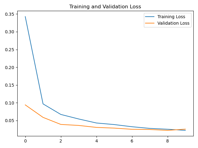
# 绘制loss曲线
plt.plot(loss, label='Training Loss')
plt.plot(val_loss, label='Validation Loss')
plt.title('Training and Validation Loss')
plt.legend()
plt.show()
# 绘制acc曲线
plt.plot(accuracy, label='Training accuracy')
plt.plot(val_accuracy, label='Validation accuracy')
plt.title('Training and Validation Accuracy')
plt.legend()
plt.show()

  模型摘要

  loss曲线

  acc曲线

  从结果来看，CNN确实比LSTM更适合MNIST数据集的分类。