- 微信
- 微博
  
  分享文章到微博
- 复制链接
  
  复制链接到剪贴板

Percolation: Slipping through the Cracks

用户已注销发表于 2022/08/17 22:59:02 2022/08/17

【摘要】目录一，二叉树场景 1，求存在长度为n的路径的概率的递推式 2，根据递推式，用不动点法求极限二，阿米巴的生存三，网格图场景 1，问题背景 2，感性认知原文链接：AMS :: Feature Column from the AMS 在一个无限大的图中，每条边都有p的概率是可通行的，有1-p的概率是不可通...

原文链接：AMS :: Feature Column from the AMS

在一个无限大的图中，每条边都有p的概率是可通行的，有1-p的概率是不可通行的，问从起点出发存在无限长路径的概率。

一，二叉树场景

Let's begin with a simple example that illustrates some general principles. We will study percolation on the infinite binary tree, a portion of which is shown below.

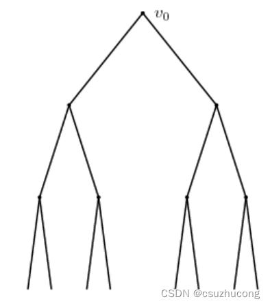
在一个无限大的二叉树中，每条边都有p的概率是可通行的，有1-p的概率是不可通行的，问从根节点出发存在无限长路径的概率。

1，求存在长度为n的路径的概率的递推式

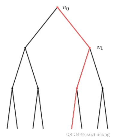
If p is the probability that each edge is open, we want to find θ(p), the probability that there is an infinite open path containing the root of the tree v0. We begin by letting Pn be the probability that there is an open path from v0 to a vertex n levels below. Notice that we have P0 = 1. Shown in red below is a path from v0 to a vertex three levels below.

This path moves through another vertex v1. The probability that an open path from v0 to a vertex n levels below passes through v1 is pPn-1, the probability p that the edge from v0 to v1 is open times the probability Pn-1 that a path from v1 to a vertex n - 1 levels below it is open. Therefore, the probability that there is no open path from v0 to a vertex n levels below passing through v1 is 1 - pPn-1.

Since any path from v0 to a vertex n levels below must pass through one of the children of v0, we find that the probability that there is not an open path from v0 to a vertex n levels below is $(1-pP_{n-1})^2$

至此，我们就得到递推式 $P_n = (1-pP_{n-1})^2$

2，根据递推式，用不动点法求极限

If we define the function fp(x) = 1 - (1 - px)2, we have Pn = fp(Pn-1). The graph of fp is shown below in two different cases, depending on the derivative fp'(0) = 2p.

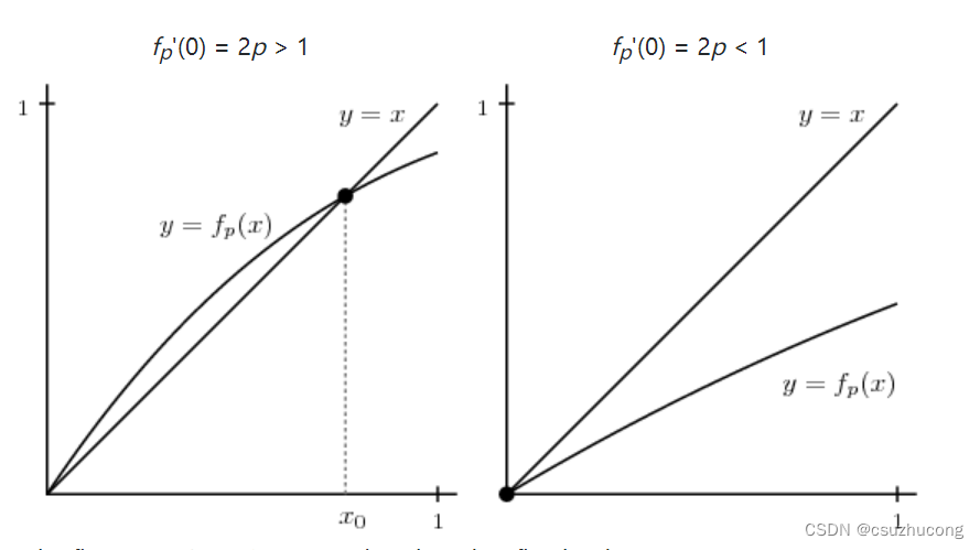
In the first case, 2p > 1 , we see that there is a fixed point

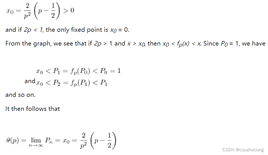
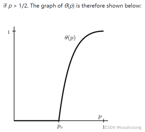
Here we see that the critical probability, pc = 1/2; above pc, θ(p) > 0 and we have percolation. Below the critical probability, θ(p) = 0 and there is no percolation.

结论就是上面的分段函数θ(p) ，p大于1/2时有概率θ(p) 存在无限长路径，p小于1/2时存在无限长路径的概率为0

This example is unusual in that it is difficult to compute the critical probability and θ(p) exactly for most combinatorial graphs. As we'll see toward the end of this article, however, it is thought that the specific form that θ(p) takes here shares features with that from other graphs.

二，阿米巴的生存

原文链接

在每一代的繁殖中，单个的阿米巴原虫有3/4的概率分裂成两个，有1/4的概率死亡（而不产生下一代）。初始时只有一个阿米巴原虫，求阿米巴原虫会无限繁殖下去的概率。

这个问题和Percolation问题的二叉树场景并不完全相同，但是非常相似。

令p为单个阿米巴原虫分裂的概率（题目中等于3/4），令P为我们要求的概率（无限繁殖的概率）。初始时的那个阿米巴原虫有p的概率分裂为两个，至少有一个可以无限生存下去的概率为1-(1-P)^2。那么，我们得到式子： P = p*( 1 – (1-P)^2 )

所以P = (2p-1)/p，p大于1/2时有概率P无限繁殖下去，p小于1/2时无限繁殖下去的概率为0

三，网格图场景

在一个无限大的网格图中，每个节点有上下左右4个邻居，即4条边，每条边都有p的概率是可通行的，有1-p的概率是不可通行的，问从起点出发存在无限长路径的概率。

1，问题背景

My backyard has an area where the soil is mainly clay and another where it's mainly sand. The day after a hard rain, the sandy region is usually dry while the clay region is still damp. The process by which water moves through a medium, like sand or clay, is called percolation and is currently the focus of significant mathematical activity, some of which we'll describe in this article.

Geoffrey Grimmett begins his book Percolation with the question: "Suppose we immerse a large porous stone in a bucket of water. What is the probability that the centre of the stone is wetted?" To begin creating a mathematical model, we will imagine a two-dimensional lattice of channels running through the rock (a more realistic three-dimensional model can wait).

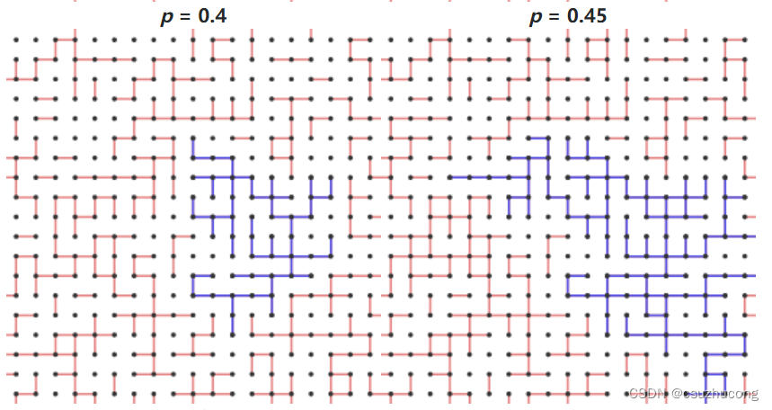
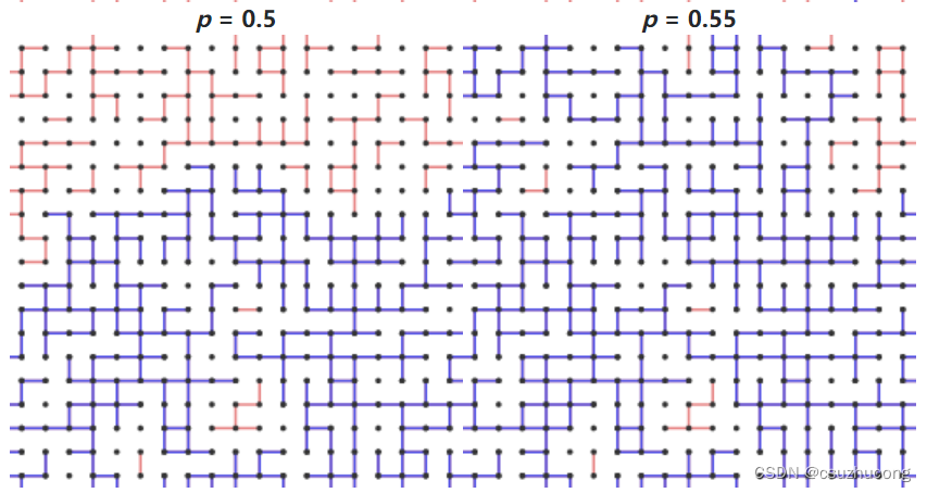
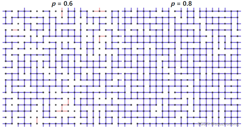
This is known as the square lattice, and we will denote it by Z2. We choose a parameter p between 0 and 1 and declare that each edge is open with probability p. Think of an open edge as a channel that is large enough to conduct water through it. Here are examples for two different values of p.

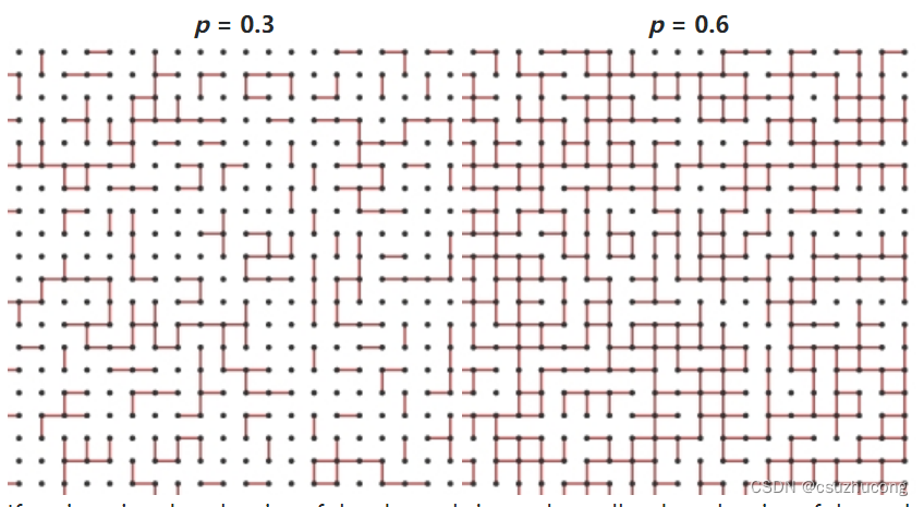
If we imagine that the size of the channels is much smaller than the size of the rock, it is reasonable to assume that the lattice is infinite in extent. To rephrase Grimmett's question, we may ask, "What is the probability that there is a path of open edges from the origin that travels infinitely far?

We can easily make two statements. When p = 0, every edge is closed so there will be no infinite open path containing the origin. However, when p = 1, every edge will be open so there must be an infinite open path.

What happens for intermediate values of p? For small p, there will be few open channels so any open paths will most likely be short. However, as p increases, there are more open channels, and eventually it is likely that there is an infinite open path starting at the origin. If there is a positive probability of having such an infinite path, we say that percolation occurs. We will see that there is a critical probability, that we denote pc, representing a threshold; percolation occurs above pc but not below. A result due to Harris and Kesten, which we'll outline later, states that the critical probability for the square lattice is pc = 1/2.

The existence of a critical probability makes percolation a mathematically interesting and rich subject. On either side of the critical probability, the system behaves in fundamentally different ways (as water drains easily through sandy soil but not through clay). As such, it serves as a model for more complex systems that experience a phase transition when some parameter, such as temperature, passes through a critical value. Percolation provides a model that is simple enough to be mathematically accessible while still displaying many of the features of more complex systems.

Percolation theory was introduced to mathematicians by Broadbent and Hammersley in 1957. For two decades, work in this new field concentrated mainly on finding critical probabilities. For instance, Broadbent and Hammersley showed that the critical probability for the square lattice Z2, shown below, is between 1/3 and 2/3.

On the basis of Monte Carlo simulations, Hammersley later suggested that this probability should be 1/2. Indeed, through work of Harris and later Kesten, it was eventually proven that pc = 1/2. We will outline the proof of this theorem later.

2，感性认知

For now, let's develop a feel for how configurations behave for various values of p.

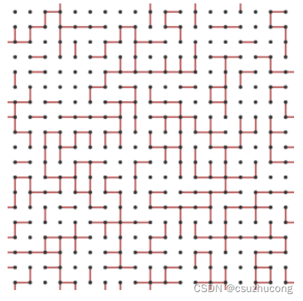
Here is one configuration of open edges that results when p = 0.4.

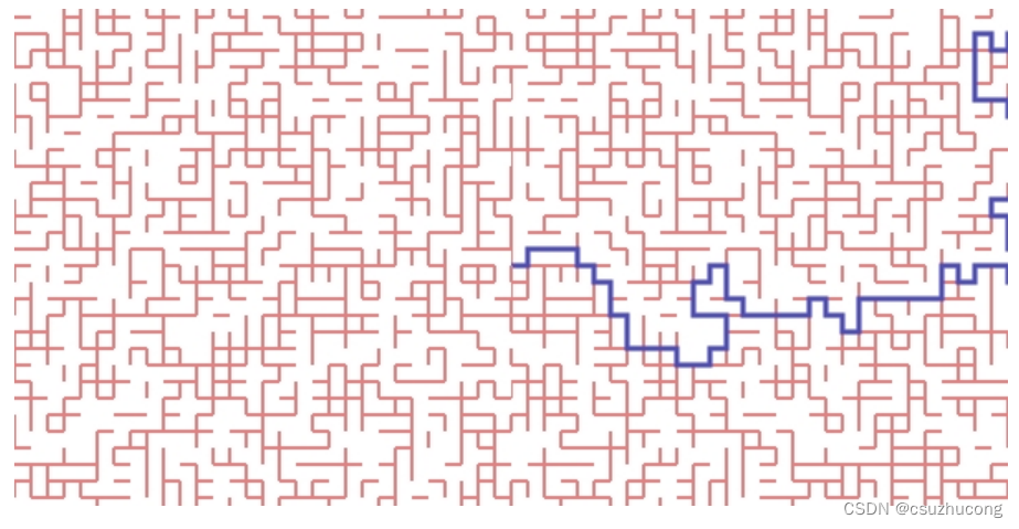
Given a configuration of open edges and a vertex v in the lattice, the cluster Cv will denote the collection of vertices connected to v by open edges.

Below we show a configuration when p = 0.3 and C0, the cluster containing the origin, in blue.

Remember that θ(p) is the probability that there is an infinite path containing the origin, which is the same event as the cluster C0 being infinite. Here's what happens as we increase p.

p=0.2