【优化覆盖】基于matlab粒子群算法优化无人机编队布局求解车载网络通信覆盖优化问题【含Matlab源码 2021期】

一、无人机简介

无人机的航迹规划是指在综合考虑无人机飞行油耗、威胁、飞行区域以及自身物理条件限制等因素的前提下, 为飞行器在飞行区域内规划出从初始点到目标点最优或者满意的飞行航迹, 其本质是一个多约束的目标优化问题。航迹规划算法是航迹规划的核心。国内外相继开展了相关研究, 提出了许多航迹规划算法, 如模拟退火算法、人工势场法、遗传算法、蚁群算法等。但由于无人机面临的规划空间异常复杂、规划约束条件多且模糊性大, 航迹搜索算法存在寻优能力差、计算量过大、效率不高等问题, 在航迹规划的最优性和实时性方面有待进一步提高。

粒子群优化算法 (particle swarm optimization, PSO)是Kennedy和Eberhart于1995年提出的一种群体智能仿生算法, 在解决一些典型的函数优化问题时, 能够取得比较好的优化结果。

1 无人机航迹规划模型
1.1 航迹表示方法
一般地, 无人机航迹规划的空间可以表示为某三维坐标系下所有点的集合{ (x, y, z) |xmin≤x≤xmax, ymin≤y≤ymax, zmin≤z≤zmax}, 其中x, y可以表示为该节点在飞行水平面下的坐标, 也可以表示为该点的经纬度, z为高程数据或海拔高度。航迹规划的目的是获得无人机在该空间中的飞行轨迹, 生成的航迹可表示为三维空间的一系列的点{PS, P1, P2, …, Pn-2, PG}, 相邻航迹点之间用直线段连接。

1.2 航迹代价函数
在航迹规划中, 常采用经过适当简化的航迹代价计算公式

式中, s表示航迹段数, Li表示第i段航迹长度, 该项代表距离代价。Hi表示第i段航迹的平均海拔高度, 该项代表高度代价。Ti为第i段航迹的威胁指数, 该项代表威胁代价。k1、k2、k3分别是距离代价、高度代价和威胁代价的权重值, 权重的选取与飞行任务要求相关。

2 基本粒子群算法
粒子群算法初始化为一群数量为N的随机粒子 (随机解) , 在D维空间中通过重复迭代、更新自身的位置以搜索适应度值最优解。粒子的位置代表被优化问题在搜索空间中的潜在解。在每次迭代中, 粒子通过跟踪2个“极值”来更新自己的速度和位置:一个是粒子自身目前所找到的最优解, 即个体极值;另一个是整个粒子群目前找到的最优解, 即全局极值。粒子i (i=1, 2, …, N) 在第j (j=1, 2, …, D) 维的速度vij和位置xij按如下格式更新:

式中, ω为非负数, 称为惯性权值 (惯性因子) , 描述了粒子对之前速度的“继承”, 即体现出粒子的“惯性”;c1和c2为非负常数, 称为学习因子 (加速因子) , 体现了粒子的社会性, 即粒子向全局最优粒子学习的特性;r1和r2为 (0, 1) 之间的随机数;pi= (pi1, pi2, …, pi D) 表示粒子i的个体极值所在位置;pg= (pg1, pg2, …, pg D) 表示所有粒子的全局极值所在位置。

速度更新公式的第一项, 反映粒子当前速度的影响, 每一个粒子按照惯性权值的比重沿着自身速度的方向搜索, 起到了平衡全局的作用, 同时避免算法陷入局部最优;第二项体现了个体最优值对粒子速度的影响, 即粒子本身的记忆和认识, 使得粒子具有全局搜索能力。第三项则反映群体对个体的影响, 即群体间的信息共享起到加速收敛的作用。

三、部分源代码

function out = PSOSearch(param, position)

% Import trace file(SUMO)
filename = param.filename;
filename_obj = param.filename_obj;
filename_connec = param.filename_connec;

% Number of vehicles available in the dataset(SUMO)
nVehicle = param.nVehicle; % Have to change according to the trace file
niter =param.niter;

% Infrastructure Position
pos = position; % Have to change according to the trace file
infRadius = 500;

% Reading table
T = readtable(filename);
T_obj = readtable(filename_obj);
T_connec = readtable(filename_connec);
% Number of rows in the table
n_rows_obj = height(T_obj);

% Finding minimum and maximum of Position X and Y
minPosX = min(T{:,4});
minPosY = min(T{:,5});
maxPosX = max(T{:,4});
maxPosY = max(T{:,5});

% Vehicle template
empty_vehicle.id = [];
empty_vehicle.Position = [];
empty_vehicle.angle = [];

% Creating templates for storing Previous connectivity history of vehicles
empty_pre_conection.id = [];
empty_pre_conection.id1 = [];
empty_pre_conection.t1 = 0;
empty_pre_conection.id2 = [];
empty_pre_conection.t2 = 0;
empty_pre_conection.id3 = [];
empty_pre_conection.t3 = 0;
empty_pre_conection.id4 = [];
empty_pre_conection.t4 = 0;
empty_pre_conection.id5 = [];
empty_pre_conection.t5 = 0;

% Create vehicles connections history array
pre_conection = repmat(empty_pre_conection, nVehicle, 1);

% Create vehicles array
object_vehicle = repmat(empty_vehicle, nVehicle, 1);
for i=1:n_rows_obj
    for j=1:nVehicle
        if strcmp(T_obj{i,1},['veh' num2str((j-1),'%d')])
            object_vehicle(j).id = T_obj{i,1};
            object_vehicle(j).angle = T_obj{i,2};
            object_vehicle(j).Position = [T_obj{i,3}, T_obj{i,4}];
        end
    end
end

% Creating vehicles id for 'connection history' data structure
for i=1:nVehicle
    pre_conection(i).id = ['veh' num2str((i-1), '%d')];
    pre_conection(i).id1 = T_connec{i,1};
    pre_conection(i).t1 = T_connec{i,2};
    pre_conection(i).id2 = T_connec{i,3};
    pre_conection(i).t2 = T_connec{i,4};
    pre_conection(i).id3 = T_connec{i,5};
    pre_conection(i).t3 = T_connec{i,6};
    pre_conection(i).id4 = T_connec{i,7};
    pre_conection(i).t4 = T_connec{i,8};
    pre_conection(i).id5 = T_connec{i,9};
    pre_conection(i).t5 = T_connec{i,10};
end

% Storing available vehicle's position in this time-slot (For scatter
% ploting only)
counter = 1;
for i=1:nVehicle
    if ~isempty(object_vehicle(i).id)
        x(counter) = object_vehicle(i).Position(1);
        y(counter) = object_vehicle(i).Position(2);
        all_vehicle(counter).id = object_vehicle(i).id;
        all_vehicle(counter).angle = object_vehicle(i).angle;
        all_vehicle(counter).Position = object_vehicle(i).Position;
        all_vehicle(counter).x = object_vehicle(i).Position(1);
        all_vehicle(counter).y = object_vehicle(i).Position(2);
        all_vehicle(counter).connec_sum = pre_conection(i).t1 + pre_conection(i).t2 + pre_conection(i).t3 ...
            + pre_conection(i).t4 + pre_conection(i).t5;
        counter = counter + 1;
    end
end

% Number of vehicles both covered and uncovered
uncovered_vehicle = all_vehicle;
nall_vehicle = size(uncovered_vehicle, 2);
counter1 = 1;

% Finding all the uncovered vehicles
for j = 1:niter
    for i = 1:nall_vehicle
        dist(j).inf = sqrt(sum((pos(j).inf - uncovered_vehicle(i).Position) .^2));
        if dist(j).inf > infRadius
            uncovered_vehicle(counter1).id = uncovered_vehicle(i).id;
            uncovered_vehicle(counter1).angle = uncovered_vehicle(i).angle;
            uncovered_vehicle(counter1).Position = uncovered_vehicle(i).Position;
            uncovered_vehicle(counter1).connec_sum = uncovered_vehicle(i).connec_sum;
            counter1 = counter1 + 1;
        end
    end
    uncovered_vehicle = uncovered_vehicle(1:counter1-1);
    nall_vehicle = size(uncovered_vehicle, 2);
    counter1 = 1;
end

% Number of uncovered vehicles
nuncovered_vehicle = size(uncovered_vehicle, 2);

% Problem Definition
nVar = 2;   % Decision Variable
VarSize = [1 nVar]; % Matrix Size of Decision Variables
VarMin = min(minPosX, minPosY);   % Lower Bound of Decision Variables
VarMax = max(maxPosX, maxPosY);    % Upper Bound of Decision Variables

% Parameters of PSO
MaxIt = param.MaxIt;    % Maximum Number of Iterations
nPop = param.nPop;  % Population Size
w = 1;      % Intertia Coefficient
wdamp = 0.99; % Damping Ratio of Intertia Coefficient
c1 = 2;     % Personal Acceleration Coefficient
c2 = 2;     % Social Acceleration Coefficient
MaxVelocity = 0.15*(VarMax-VarMin);
MinVelocity = -MaxVelocity;

% Initialization
% The particle template
empty_particle.Position = [];
empty_particle.Velocity = [];
empty_particle.Cost = [];
empty_particle.Best.Position = [];
empty_particle.Best.Cost = [];

% create population array
particle = repmat(empty_particle, nPop, 1);

% Initialize Global Best
GlobalBest.Cost = -inf;
GlobalBest.Position = [0,0];

% Initialize population members
for i=1:nPop
    % Generate Random Solution
  

    % Initialize Velociy
    particle(i).Velocity = zeros(VarSize);

    % Evaluation
    evaluation = objfuntest(particle(i).Position, nuncovered_vehicle, uncovered_vehicle, pos, niter);
    particle(i).Cost = evaluation.Fitness;
    nMi = evaluation.M;
    nNi = evaluation.N;

    % Update the Personal Best
    particle(i).Best.Position = particle(i).Position;
    particle(i).Best.Cost = particle(i).Cost;

    % Update Global Best
    if particle(i).Best.Cost > GlobalBest.Cost
     
end
% Array to Hold Best Cost Value on Each Iteration
BestCosts = zeros(MaxIt, 1);

nM = 0;
nN = 0;

%  Main Loop of PSO
for it=1:MaxIt
    for i=1:nPop
        % Update Velocity
        particle(i).Velocity = w*particle(i).Velocity ...
            + c1*rand(VarSize).*(particle(i).Best.Position - particle(i).Position) ...
            + c2*rand(VarSize).*(GlobalBest.Position -particle(i).Position);

        % Apply Velocity Limits
        particle(i).Velocity = max(particle(i).Velocity, MinVelocity);
        particle(i).Velocity = min(particle(i).Velocity, MaxVelocity);

        % Update Position
        particle(i).Position = particle(i).Position + particle(i).Velocity;

        % Apply Lower and Upper Bound Limits
        particle(i).Position = max(particle(i).Position, VarMin);
        particle(i).Position = min(particle(i).Position, VarMax);

        % Evaluation
        evaluation = objfuntest(particle(i).Position, nuncovered_vehicle, uncovered_vehicle, pos, niter);
        particle(i).Cost = evaluation.Fitness;

        % Update Personal Best
        if particle(i).Cost > particle(i).Best.Cost

        
        end
    end
    % Store the Best Cost Value
    BestCosts(it) = GlobalBest.Cost;

    % Damping Intertia Coefficient
    w = w * wdamp;
end
out.Fitness = GlobalBest.Cost;
out.Position = GlobalBest.Position;
out.Uncov_veh = evaluation.V;
out.nM = nM;
out.nN = nN;
out.x = x;
out.y = y;
out.VarMin = VarMin;
out.VarMax = VarMax;
out.Total_vehicle = size(all_vehicle, 2);
out.Best_cost = BestCosts;

  

 

  
 
 

  
1
  
2
  
3
  
4
  
5
  
6
  
7
  
8
  
9
  
10
  
11
  
12
  
13
  
14
  
15
  
16
  
17
  
18
  
19
  
20
  
21
  
22
  
23
  
24
  
25
  
26
  
27
  
28
  
29
  
30
  
31
  
32
  
33
  
34
  
35
  
36
  
37
  
38
  
39
  
40
  
41
  
42
  
43
  
44
  
45
  
46
  
47
  
48
  
49
  
50
  
51
  
52
  
53
  
54
  
55
  
56
  
57
  
58
  
59
  
60
  
61
  
62
  
63
  
64
  
65
  
66
  
67
  
68
  
69
  
70
  
71
  
72
  
73
  
74
  
75
  
76
  
77
  
78
  
79
  
80
  
81
  
82
  
83
  
84
  
85
  
86
  
87
  
88
  
89
  
90
  
91
  
92
  
93
  
94
  
95
  
96
  
97
  
98
  
99
  
100
  
101
  
102
  
103
  
104
  
105
  
106
  
107
  
108
  
109
  
110
  
111
  
112
  
113
  
114
  
115
  
116
  
117
  
118
  
119
  
120
  
121
  
122
  
123
  
124
  
125
  
126
  
127
  
128
  
129
  
130
  
131
  
132
  
133
  
134
  
135
  
136
  
137
  
138
  
139
  
140
  
141
  
142
  
143
  
144
  
145
  
146
  
147
  
148
  
149
  
150
  
151
  
152
  
153
  
154
  
155
  
156
  
157
  
158
  
159
  
160
  
161
  
162
  
163
  
164
  
165
  
166
  
167
  
168
  
169
  
170
  
171
  
172
  
173
  
174
  
175
  
176
  
177
  
178
  
179
  
180
  
181
  
182
  
183
  
184
  
185
  
186
  
187
  
188
  
189
  
190
  
191
  
192
  
193
  
194
  
195
  
196
  
197
  
198
  
199
  
200
  
201
  
202
  
203
  
204
  
205
  
206
  
207
  
208
  
209
  
210
  
211
  
212
  
213
  
214
  
215
  
216
  
217
  
218
  
219
  
220
  
221
  
222
 

end

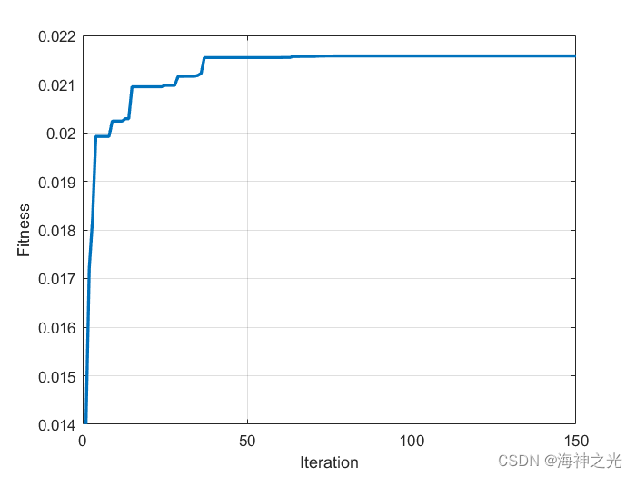
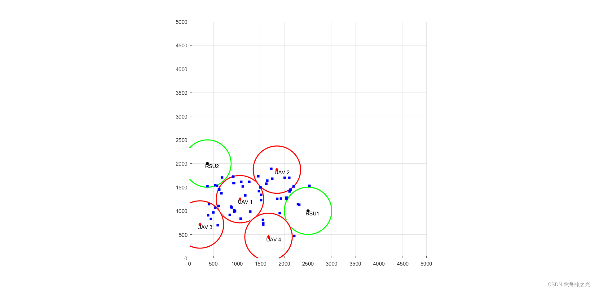
四、运行结果

五、matlab版本及参考文献

1 matlab版本
2014a

2 参考文献
[1] 包子阳,余继周,杨杉.智能优化算法及其MATLAB实例（第2版）[M].电子工业出版社，2016.
[2]张岩,吴水根.MATLAB优化算法源代码[M].清华大学出版社，2017.
[3]巫茜,罗金彪,顾晓群,曾青.基于改进PSO的无人机三维航迹规划优化算法[J].兵器装备工程学报. 2021,42(08)
[4]方群,徐青.基于改进粒子群算法的无人机三维航迹规划[J].西北工业大学学报. 2017,35(01)

文章来源: qq912100926.blog.csdn.net，作者：海神之光，版权归原作者所有，如需转载，请联系作者。

原文链接：qq912100926.blog.csdn.net/article/details/126178366