【心电信号】基于matlab心率检测【含Matlab源码 1993期】

一、心电信号简介

0 引言
心电信号是人类最早研究的生物信号之一, 相比其他生物信号更易于检测, 且具有直观的规律。心电图的准确分析对心脏病的及早治疗有重大的意义。人体是一个复杂精密的系统, 有许多不可抗的外界因素, 得到纯净的心电信号非常困难。可以采用神经网络算法去除心电信号的噪声, 但这种方法存在训练难度大、耗时长的缺点。小波变换在处理非线性、非平稳且奇异点较多的信号时具有一定的优越性, 近年来许多学者使用其对心电信号进行研究。

1 心电信号简介
心电信号由以下几个波段组成, 一个典型的心电图如图1所示。

图1 典型心电图
(1) P波:反映心房肌在除极过程中的电位变化过程;
(2) P-R间期:反映的是激动从窦房结通过房室交界区到心室肌开始除极的时限;
(3) QRS波群:反映心室肌除极过程的电位变化;
(4) T波:代表心室肌复极过程中所引起的电位变化;
(5) S-T段:从QRS波群终点到达T波起点间的一段水平线[2];
(6) Q-T间期:心室从除极到复极的时间[3];
(7) U波:代表动作电位的后电位。
由于心电信号十分微弱, 且低频, 极易受到干扰, 不同的干扰源的噪声虽是随机的, 但来自同一个干扰源的噪声往往具有同一类特征。分析干扰的来源, 针对不同的来源使用合适的处理方法, 是数据采集重点考虑的一个问题。常见干扰有3种: (1) 工频干扰; (2) 基线漂移; (3) 肌电干扰。其中已经证明小波变换在抑制心电信号的工频干扰方面具有较大优势。具体噪声频带如表1所示。
表1 心电信号以及主要噪声频带

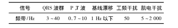
二、部分源代码

function main
%MAIN creates Figure 4, Figure 5 and Figure 6 in the paper.

%% Load the data and constrruct the simulated ta-ECG signals
load 'fECG.mat';
load 'mECG.mat';

% Preprocessing (removing the mean, normalizing by the maximum, removing
% the net noise (60Hz) and median filtering):
fs = 250;
fECG = bsxfun(@minus,   fECG, mean(fECG));
fECG = bsxfun(@rdivide, fECG, 0.5*max(fECG));
mECG = bsxfun(@minus,   mECG, mean(mECG));
mECG = bsxfun(@rdivide, mECG, 0.5*max(mECG));

notchFilt = fdesign.notch(4,60/(fs/2),1);
Hnotch    = design(notchFilt);
fECG(:,2) = filter(Hnotch,fECG(:,2) - medfilt1(fECG(:,2),100));
fECG(:,3) = filter(Hnotch,fECG(:,3) - medfilt1(fECG(:,3),100));
mECG(:,3) = filter(Hnotch,mECG(:,3) - medfilt1(mECG(:,3),100));

% Upsampling the ECG representing the maternal signal by a factor of 4 and
% the ECG representing the fetal signal by a factor of 2 (fECG will be
% approximately 2 times faster than mECG)
mECGrs  = resample(mECG(:,3), 4, 1);
fECGrs1 = resample(fECG(:,2), 2, 1); 
fECGrs2 = resample(fECG(:,3), 2, 1); 
fs = 1000;

% Constructing the ta-ECG signals:
len = 40000; % Number of samples to use in the analysis
sig_range = 1:len;
sig1 = 2*mECGrs(sig_range) -     fECGrs1(sig_range);
sig2 =   mECGrs(sig_range) - 0.5*fECGrs2(sig_range);

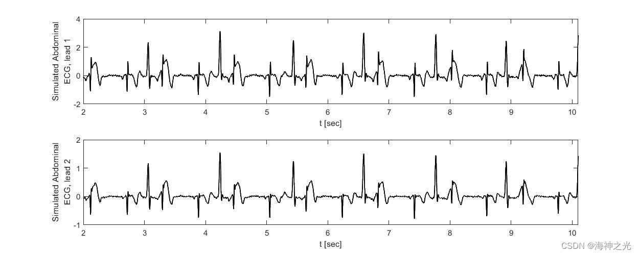
% Plotting Figure 4:
figure('Name','Figure 4'); 
lx(1) = subplot(2,1,1); plot(0:1/fs:(len/fs-1/fs),sig1,'k','LineWidth',1); xlabel('t [sec]'); ylabel({'Simulated Abdominal' ; 'ECG, lead 1'})
lx(2) = subplot(2,1,2); plot(0:1/fs:(len/fs-1/fs),sig2,'k','LineWidth',1); xlabel('t [sec]'); ylabel({'Simulated Abdominal' ; 'ECG, lead 2'})
linkaxes(lx,'x');
xlim([2,10.1]);
set(gcf,'Position',[800,400,1000,400]);

%% Construct a lagmap of the signal and reference data and construct the ground truth signals

lag  = 12;
jump = lag/2;

% Lagmap of the ta-ECG simulated signals:
siglag1 = const_lag( sig1, lag, jump );
siglag2 = const_lag( sig2, lag, jump );

% Reference data lagmaps:
fECGmean = mean( const_lag( fECGrs1(sig_range), lag, jump ), 2); 
% fECG values at points that will correspond to the eigenvector points of 
% the diffusion maps operators and operators A and S

mECGmean = mean( const_lag( mECGrs(sig_range), lag, jump ), 2); 
% fECG values at points that will correspond to the eigenvector points of 
% the diffusion maps operators and operators A and S

% Ground truth of fECG beat locations and mECG beat locations:
fECGgt = fECGrs2(sig_range);
fECGgt = fECGgt>1;
fECGgt = sum( const_lag( fECGgt, lag, jump ), 2);
fECGgt(fECGgt>0) = 1;

mECGgt = mECGrs(sig_range);
mECGgt = mECGgt>1;
mECGgt = sum( const_lag( mECGgt, lag, jump ), 2);
mECGgt(mECGgt>0) = 1;

%% Calculate the diffusion maps kernels and eigenvectors
ep = 1;

[ V1, ~, K1 ] = dm( siglag1, ep );
[ V2, ~, K2 ] = dm( siglag2, ep );

%% Constructing the operators S and A and their eigenvectors

S = K1*K2.' + K2*K1.';
A = K1*K2.' - K2*K1.';

[VS, ES] = eigs(S,10);
[~, I]   = sort(real(diag(ES)),'descend');
VS       = real(VS(:,I));

[VA, EA] = eigs(A,10);
[~, I]   = sort(imag(diag(EA)),'descend');
VA       = VA(:,I);

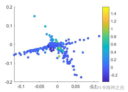
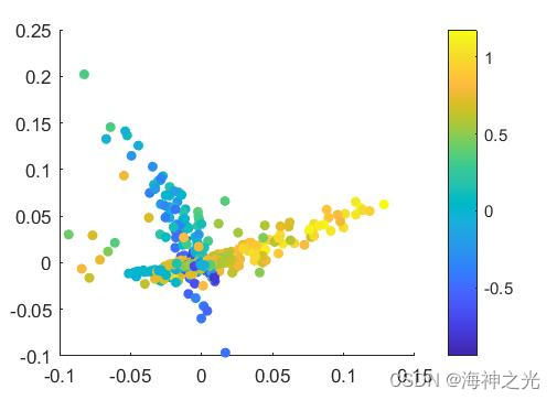
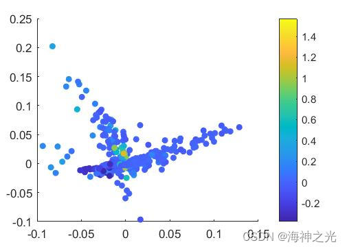
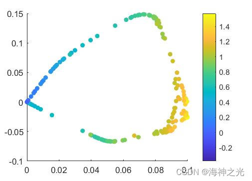
%% Plotting Figure 5

fig5( V1, V2, VS, VA, mECGmean, fECGmean )

%% Plotting Figure 6


x = [(1:length(fECGmean))*jump/fs; (1:length(fECGmean))*jump/fs];
y = [pltsig1(:).'; pltsig1(:).'];
z = zeros(size(y));

c = [double((abs((VS(:,2))).')>1e-2); double((abs((VS(:,2))).')>1e-2)];
figure('Name','ta-ECG colored by a thresholded eigenvector of S')
surface(x,y,z,c,'facecolor','none','edgecolor','flat','LineWidth',2); colormap(cmap);
ax1 = gca;
yl = ax1.YLim;
hold on
line(repmat(find((mECGgt>0).')*jump/fs,10,1),repmat(linspace(yl(1),yl(2),10).',1,sum(mECGgt)),'Color' ,[0.3,0.3,0.3,0.3], 'LineStyle',':','LineWidth',1.5)
xlabel('t [sec]');
set(ax1,'YTick',[])
xlim([12.2,22.2]);
hold off;
set(gcf,'Position',[600,500,1200,250]);

c = [double((abs(imag(VA(:,2))).')>3e-2); double((abs(imag(VA(:,2))).')>3e-2)];
figure('Name','ta-ECG colored by a thresholded eigenvector of A')
surface(x,y,z,c,'facecolor','none','edgecolor','flat','LineWidth',2); colormap(cmap);
ax2 = gca;
yl = ax2.YLim;
hold on
line(repmat(find((fECGgt>0).')*jump/fs,10,1),repmat(linspace(yl(1),yl(2),10).',1,sum(fECGgt)),'Color' ,[0.3,0.3,0.3,0.3], 'LineStyle','--','LineWidth',1)
xlabel('t [sec]');
set(ax2,'YTick',[])
xlim([12.2,22.2]);
hold off;
set(gcf,'Position',[600,200,1200,250]);

linkaxes([ax1,ax2],'xy')

end


  

 

  
 
 

  
1
  
2
  
3
  
4
  
5
  
6
  
7
  
8
  
9
  
10
  
11
  
12
  
13
  
14
  
15
  
16
  
17
  
18
  
19
  
20
  
21
  
22
  
23
  
24
  
25
  
26
  
27
  
28
  
29
  
30
  
31
  
32
  
33
  
34
  
35
  
36
  
37
  
38
  
39
  
40
  
41
  
42
  
43
  
44
  
45
  
46
  
47
  
48
  
49
  
50
  
51
  
52
  
53
  
54
  
55
  
56
  
57
  
58
  
59
  
60
  
61
  
62
  
63
  
64
  
65
  
66
  
67
  
68
  
69
  
70
  
71
  
72
  
73
  
74
  
75
  
76
  
77
  
78
  
79
  
80
  
81
  
82
  
83
  
84
  
85
  
86
  
87
  
88
  
89
  
90
  
91
  
92
  
93
  
94
  
95
  
96
  
97
  
98
  
99
  
100
  
101
  
102
  
103
  
104
  
105
  
106
  
107
  
108
  
109
  
110
  
111
  
112
  
113
  
114
  
115
  
116
  
117
  
118
  
119
  
120
  
121
  
122
  
123
  
124
  
125
  
126
  
127
  
128
  
129
  
130
  
131
  
132
 

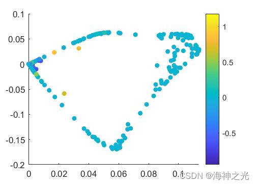
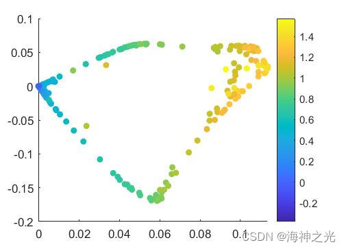
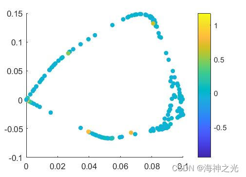
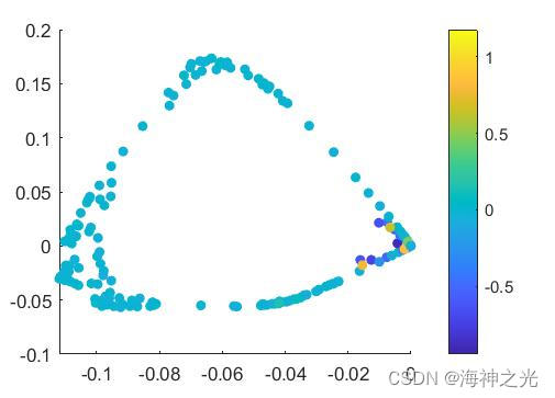
三、运行结果

四、matlab版本及参考文献

1 matlab版本
2014a

2 参考文献
[1] 沈再阳.精通MATLAB信号处理[M].清华大学出版社，2015.
[2]高宝建,彭进业,王琳,潘建寿.信号与系统——使用MATLAB分析与实现[M].清华大学出版社，2020.
[3]王文光,魏少明,任欣.信号处理与系统分析的MATLAB实现[M].电子工业出版社，2018.
[4]焦运良，邢计元，靳尧凯.基于小波变换的心电信号阈值去噪算法研究[J].信息技术与网络安全. 2019,38(05)

文章来源: qq912100926.blog.csdn.net，作者：海神之光，版权归原作者所有，如需转载，请联系作者。

原文链接：qq912100926.blog.csdn.net/article/details/126077251