- 微信
- 微博
  
  分享文章到微博
- 复制链接
  
  复制链接到剪贴板

【物理应用】基于matlab双目视觉三维重建【含Matlab源码 1781期】

海神之光发表于 2022/05/30 01:02:42 2022/05/30

【摘要】一、获取代码方式获取代码方式1：完整代码已上传我的资源：【物理应用】基于matlab双目视觉三维重建【含Matlab源码 1781期】获取代码方式2：通过订阅紫极神光博客付费专栏，凭支付凭证，...

一、获取代码方式

获取代码方式1：
完整代码已上传我的资源：【物理应用】基于matlab双目视觉三维重建【含Matlab源码 1781期】

获取代码方式2：
通过订阅紫极神光博客付费专栏，凭支付凭证，私信博主，可获得此代码。

备注：
订阅紫极神光博客付费专栏，可免费获得1份代码（有效期为订阅日起，三天内有效）；

二、部分源代码

%% Clean the slate
% The demo here in the main.html document can be run directly from main.m
% In this section the memory is cleared, some parameters are set, and the
% original images are loaded and displayed.
close all
clear
clc

% Setting up parameters and filenames
params.VERBOSE          = 1;                    %Get more plots out (True or False)
params.PLANE            = 3;                    %Which plane of the RGB is of interest to us for opperations on a single plane
params.BLACK_BACKGROUND = 1;                    %Images have a black background (True or False)
params.map                      = copper(256);  %Set colormap to something that is similar to wood
params.number_angular_divisions = 2^7;          %Powers of two are faster FFT
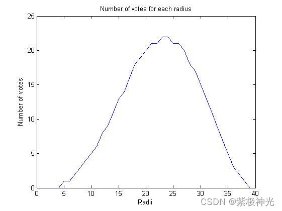
params.number_radial_divisions  = 40;           %Arbitrary constant
base_filename = 'dowel01.jpg';                  %Filename of non-moving image  
move_filename = 'dowel02.jpg';                  %Filename of image that will move to the base image

base_image = imread(base_filename);    %reads in the image
move_image = imread(move_filename);    %reads in the image

% Data visualization.  
subplot(1,2,1)                    
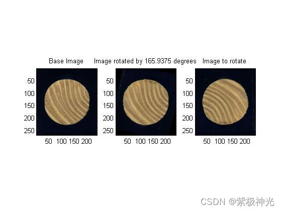
subimage(base_image);          
title('Base image') 
subplot(1,2,2)                    
subimage(move_image);          
title('Image to move')
set (gcf, 'color', 'w')

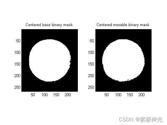
%% Correct the X and Y displacements
% The two images are displaced from each other in the X and Y direcions.
% First the X and Y direction will be corrected by lining up the centroids
% of the two images.
%
% Method: First mask the image from background then find
% centroid of the image. Finally center the image based 
% on its centroid.

base_plane_of_interest              = base_image(:,:,params.PLANE);
%Must use a single layer grayscale for most operations.  Blue plane is best
%contrast for these images
base_bw_plane_of_interest           = im2bw(base_plane_of_interest, graythresh(base_plane_of_interest));
%Turn to binary based on threshold gotten from graythresh
base_plane_of_interest_segmented    = bwmorph(base_bw_plane_of_interest, 'open');
%morphology
base_binary_mask                    = imfill (base_plane_of_interest_segmented, 'holes');
%fill it in

% Get some data about the new region
base_properties                     = regionprops(real(base_binary_mask),'all');
base_centroid_row                   = round(base_properties.Centroid(2));
base_centroid_col                   = round(base_properties.Centroid(1));

% Place a dot at the centroid, one for each layer
base_image(base_centroid_row, base_centroid_col, 1) = 255;
base_image(base_centroid_row, base_centroid_col, 2) = 255;
base_image(base_centroid_row, base_centroid_col, 3) = 255;

% Nice to have image be 0dd number of pixels in each diension
base_image       = make_odd_by_odd(base_image);
base_binary_mask = make_odd_by_odd(base_binary_mask);
% Grab the new size
[base_num_rows, base_num_cols, base_num_layers] = size(base_image);

% Where is the center of the image?
base_goal_row   = (base_num_rows - 1) / 2 + 1;
base_goal_col   = (base_num_cols - 1) / 2 + 1;

% how much do I need to move to center this?
base_delta_rows = base_goal_row - base_centroid_row;
base_delta_cols = base_goal_col - base_centroid_col;

%shift the images to be centered
base_image       = circshift(base_image      , [base_delta_rows, base_delta_cols]);
base_binary_mask = circshift(base_binary_mask, [base_delta_rows, base_delta_cols]);

% Same thing for the second image.  In production code this would be in 
% a function, but this script was made for seminar presentation where all
% the code should be visible.
% Begin repeated code -------------------------------------
move_plane_of_interest              = move_image(:,:,params.PLANE);
move_bw_plane_of_interest           = im2bw(move_plane_of_interest, graythresh(move_plane_of_interest));
move_plane_of_interest_segmented    = bwmorph(move_bw_plane_of_interest, 'open');
move_binary_mask                    = imfill (move_plane_of_interest_segmented, 'holes');
move_properties                     = regionprops(real(move_binary_mask),'all');
move_centroid_row                   = round(move_properties.Centroid(2));
move_centroid_col                   = round(move_properties.Centroid(1));
move_image(move_centroid_row, move_centroid_col, 1) = 255;
move_image(move_centroid_row, move_centroid_col, 2) = 255;
move_image(move_centroid_row, move_centroid_col, 3) = 255;
move_image                          = make_odd_by_odd(move_image);
move_binary_mask                    = make_odd_by_odd(move_binary_mask);
[move_num_rows, move_num_cols, move_num_layers]     = size(move_image);
move_goal_row                       = (move_num_rows - 1) / 2 + 1;
move_goal_col                       = (move_num_cols - 1) / 2 + 1;
move_delta_rows                     = move_goal_row - move_centroid_row;
move_delta_cols                     = move_goal_col - move_centroid_col;
move_image                          = circshift(move_image      , [move_delta_rows, move_delta_cols]);
move_binary_mask                    = circshift(move_binary_mask, [move_delta_rows, move_delta_cols]);
% End of repeated code -------------------------------------

% Data visualization
subplot(1,2,1)                    
subimage(base_image);
title('Centered base image') 
subplot(1,2,2)                    
subimage(move_image);          
title('Centered moveable image')
set (gcf, 'color', 'w')

  
 
  1
  2
  3
  4
  5
  6
  7
  8
  9
  10
  11
  12
  13
  14
  15
  16
  17
  18
  19
  20
  21
  22
  23
  24
  25
  26
  27
  28
  29
  30
  31
  32
  33
  34
  35
  36
  37
  38
  39
  40
  41
  42
  43
  44
  45
  46
  47
  48
  49
  50
  51
  52
  53
  54
  55
  56
  57
  58
  59
  60
  61
  62
  63
  64
  65
  66
  67
  68
  69
  70
  71
  72
  73
  74
  75
  76
  77
  78
  79
  80
  81
  82
  83
  84
  85
  86
  87
  88
  89
  90
  91
  92
  93
  94
  95
  96
  97
  98
  99
  100
  101
  102
  103
  104
  105
  106
  107
  108
  109
  110