【优化布局】基于matlab遗传算法求解带出入点的车间布局优化问题【含Matlab源码 011期】

一、遗传算法简介

1 遗传算法概述
遗传算法（Genetic Algorithm，GA）是进化计算的一部分，是模拟达尔文的遗传选择和自然淘汰的生物进化过程的计算模型，是一种通过模拟自然进化过程搜索最优解的方法。该算法简单、通用，鲁棒性强，适于并行处理。

2 遗传算法的特点和应用
遗传算法是一类可用于复杂系统优化的具有鲁棒性的搜索算法，与传统的优化算法相比，具有以下特点：
（1）以决策变量的编码作为运算对象。传统的优化算法往往直接利用决策变量的实际值本身来进行优化计算，但遗传算法是使用决策变量的某种形式的编码作为运算对象。这种对决策变量的编码处理方式，使得我们在优化计算中可借鉴生物学中染色体和基因等概念，可以模仿自然界中生物的遗传和进化激励，也可以很方便地应用遗传操作算子。
（2）直接以适应度作为搜索信息。传统的优化算法不仅需要利用目标函数值，而且搜索过程往往受目标函数的连续性约束，有可能还需要满足“目标函数的导数必须存在”的要求以确定搜索方向。遗传算法仅使用由目标函数值变换来的适应度函数值就可确定进一步的搜索范围，无需目标函数的导数值等其他辅助信息。直接利用目标函数值或个体适应度值也可以将搜索范围集中到适应度较高部分的搜索空间中，从而提高搜索效率。
（3）使用多个点的搜索信息，具有隐含并行性。传统的优化算法往往是从解空间的一个初始点开始最优解的迭代搜索过程。单个点所提供的搜索信息不多，所以搜索效率不高，还有可能陷入局部最优解而停滞；遗传算法从由很多个体组成的初始种群开始最优解的搜索过程，而不是从单个个体开始搜索。对初始群体进行的、选择、交叉、变异等运算，产生出新一代群体，其中包括了许多群体信息。这些信息可以避免搜索一些不必要的点，从而避免陷入局部最优，逐步逼近全局最优解。
（4） 使用概率搜索而非确定性规则。传统的优化算法往往使用确定性的搜索方法，一个搜索点到另一个搜索点的转移有确定的转移方向和转移关系，这种确定性可能使得搜索达不到最优店，限制了算法的应用范围。遗传算法是一种自适应搜索技术，其选择、交叉、变异等运算都是以一种概率方式进行的，增加了搜索过程的灵活性，而且能以较大概率收敛于最优解，具有较好的全局优化求解能力。但，交叉概率、变异概率等参数也会影响算法的搜索结果和搜索效率，所以如何选择遗传算法的参数在其应用中是一个比较重要的问题。
综上，由于遗传算法的整体搜索策略和优化搜索方式在计算时不依赖于梯度信息或其他辅助知识，只需要求解影响搜索方向的目标函数和相应的适应度函数，所以遗传算法提供了一种求解复杂系统问题的通用框架。它不依赖于问题的具体领域，对问题的种类有很强的鲁棒性，所以广泛应用于各种领域，包括：函数优化、组合优化生产调度问题、自动控制
、机器人学、图像处理（图像恢复、图像边缘特征提取…)、人工生命、遗传编程、机器学习。

3 遗传算法的基本流程及实现技术
基本遗传算法（Simple Genetic Algorithms,SGA）只使用选择算子、交叉算子和变异算子这三种遗传算子，进化过程简单，是其他遗传算法的基础。

3.1 遗传算法的基本流程
通过随机方式产生若干由确定长度（长度与待求解问题的精度有关）编码的初始群体；
通过适应度函数对每个个体进行评价，选择适应度值高的个体参与遗传操作，适应度低的个体被淘汰；
经遗传操作（复制、交叉、变异）的个体集合形成新一代种群，直到满足停止准则（进化代数GEN>=?）；
将后代中变现最好的个体作为遗传算法的执行结果。

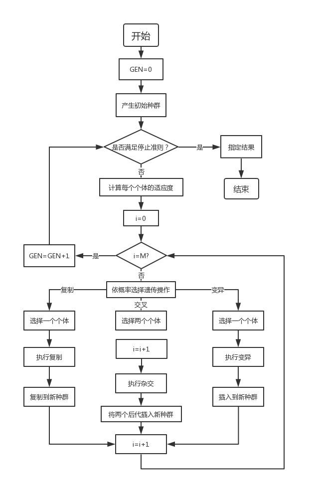
其中，GEN是当前代数；M是种群规模，i代表种群数量。

3.2 遗传算法的实现技术
基本遗传算法（SGA）由编码、适应度函数、遗传算子（选择、交叉、变异）及运行参数组成。
3.2.1 编码
（1）二进制编码
二进制编码的字符串长度与问题所求解的精度有关。需要保证所求解空间内的每一个个体都可以被编码。
优点：编、解码操作简单，遗传、交叉便于实现
缺点：长度大
（2）其他编码方法
格雷码、浮点数编码、符号编码、多参数编码等
3.2.2 适应度函数
适应度函数要有效反映每一个染色体与问题的最优解染色体之间的差距。
3.2.3选择算子

3.2.4 交叉算子
交叉运算是指对两个相互配对的染色体按某种方式相互交换其部分基因，从而形成两个新的个体；交叉运算是遗传算法区别于其他进化算法的重要特征，是产生新个体的主要方法。在交叉之前需要将群体中的个体进行配对，一般采取随机配对原则。
常用的交叉方式：
单点交叉
双点交叉（多点交叉，交叉点数越多，个体的结构被破坏的可能性越大，一般不采用多点交叉的方式）
均匀交叉
算术交叉
3.2.5 变异算子
遗传算法中的变异运算是指将个体染色体编码串中的某些基因座上的基因值用该基因座的其他等位基因来替换，从而形成一个新的个体。

就遗传算法运算过程中产生新个体的能力方面来说，交叉运算是产生新个体的主要方法，它决定了遗传算法的全局搜索能力；而变异运算只是产生新个体的辅助方法，但也是必不可少的一个运算步骤，它决定了遗传算法的局部搜索能力。交叉算子与变异算子的共同配合完成了其对搜索空间的全局搜索和局部搜索，从而使遗传算法能以良好的搜索性能完成最优化问题的寻优过程。

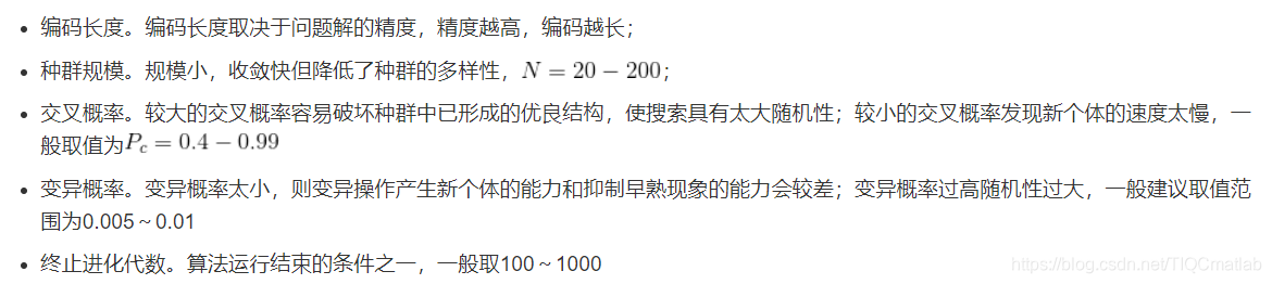
3.2.6 运行参数

4 遗传算法的基本原理
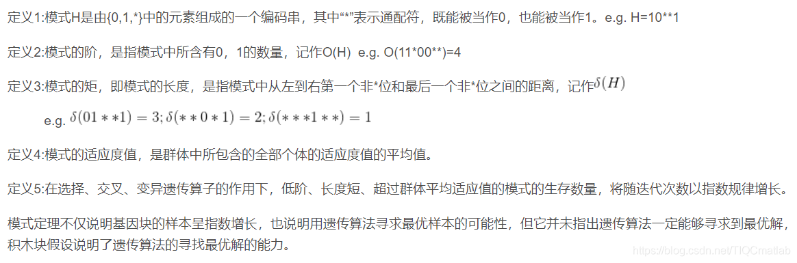
4.1 模式定理

4.2 积木块假设
具有低阶、定义长度短，且适应度值高于群体平均适应度值的模式称为基因块或积木块。
积木块假设：个体的基因块通过选择、交叉、变异等遗传算子的作用，能够相互拼接在一起，形成适应度更高的个体编码串。
积木块假设说明了用遗传算法求解各类问题的基本思想，即通过积木块直接相互拼接在一起能够产生更好的解。

二、部分源代码

clc;
clear;
close all;

%% Problem Definition

model=CreateModel();                        % Create Model

CostFunction=@(sol1) MyCost(sol1,model);	% Cost Function

Vars.xhat.Min=0;
Vars.xhat.Max=1;
Vars.xhat.Size=[1 model.n];
Vars.xhat.Count=prod(Vars.xhat.Size);
Vars.xhat.VelMax=0.1*(Vars.xhat.Max-Vars.xhat.Min);
Vars.xhat.VelMin=-Vars.xhat.VelMax;

Vars.yhat.Min=0;
Vars.yhat.Max=1;
Vars.yhat.Size=[1 model.n];
Vars.yhat.Count=prod(Vars.yhat.Size);
Vars.yhat.VelMax=0.1*(Vars.yhat.Max-Vars.yhat.Min);
Vars.yhat.VelMin=-Vars.yhat.VelMax;

Vars.rhat.Min=0;
Vars.rhat.Max=1;
Vars.rhat.Size=[1 model.n];
Vars.rhat.Count=prod(Vars.rhat.Size);
Vars.rhat.VelMax=0.1*(Vars.rhat.Max-Vars.rhat.Min);
Vars.rhat.VelMin=-Vars.rhat.VelMax;

%% PSO Parameters

MaxIt=500;      % Maximum Number of Iterations

nPop=50;        % Population Size (Swarm Size)

w=1.0;          % Inertia Weight
wdamp=0.99;     % Inertia Weight Damping Ratio
c1=0.7;         % Personal Learning Coefficient
c2=1.5;         % Global Learning Coefficient

% % Constriction Coefficients
% phi1=2.05;
% phi2=2.05;
% phi=phi1+phi2;
% chi=2/(phi-2+sqrt(phi^2-4*phi));
% w=chi;          % Inertia Weight
% wdamp=1;        % Inertia Weight Damping Ratio
% c1=chi*phi1;    % Personal Learning Coefficient
% c2=chi*phi2;    % Global Learning Coefficient


%% Initialization

empty_particle.Position=[];
empty_particle.Cost=[];
empty_particle.Sol=[];
empty_particle.Velocity=[];
empty_particle.Best.Position=[];
empty_particle.Best.Cost=[];
empty_particle.Best.Sol=[];

particle=repmat(empty_particle,nPop,1);

GlobalBest.Cost=inf;

for i=1:nPop
    
    % Initialize Position
    particle(i).Position=CreateRandomSolution(model);
    
    % Initialize Velocity
    particle(i).Velocity.xhat=zeros(Vars.xhat.Size);
    particle(i).Velocity.yhat=zeros(Vars.yhat.Size);
    particle(i).Velocity.rhat=zeros(Vars.rhat.Size);
    
    % Evaluation
    [particle(i).Cost, particle(i).Sol]=CostFunction(particle(i).Position);
    
    % Update Personal Best
    particle(i).Best.Position=particle(i).Position;
    particle(i).Best.Cost=particle(i).Cost;
    particle(i).Best.Sol=particle(i).Sol;
    
    % Update Global Best
    if particle(i).Best.Cost<GlobalBest.Cost
        GlobalBest=particle(i).Best;
    end
end

BestCost=zeros(MaxIt,1);


%% PSO Main Loop

for it=1:MaxIt
    
    for i=1:nPop
        
        % ---- Motion on xhat
        
        % Update Velocity
        particle(i).Velocity.xhat = w*particle(i).Velocity.xhat ...
            +c1*rand(Vars.xhat.Size).*(particle(i).Best.Position.xhat-particle(i).Position.xhat) ...
            +c2*rand(Vars.xhat.Size).*(GlobalBest.Position.xhat-particle(i).Position.xhat);
        
        % Apply Velocity Limits
        particle(i).Velocity.xhat = max(particle(i).Velocity.xhat,Vars.xhat.VelMin);
        particle(i).Velocity.xhat = min(particle(i).Velocity.xhat,Vars.xhat.VelMax);
        
        % Update Position
        particle(i).Position.xhat = particle(i).Position.xhat + particle(i).Velocity.xhat;
        
        % Velocity Mirror Effect
        IsOutside=(particle(i).Position.xhat<Vars.xhat.Min | particle(i).Position.xhat>Vars.xhat.Max);
        particle(i).Velocity.xhat(IsOutside)=-particle(i).Velocity.xhat(IsOutside);
        
        % Apply Position Limits
        particle(i).Position.xhat = max(particle(i).Position.xhat,Vars.xhat.Min);
        particle(i).Position.xhat = min(particle(i).Position.xhat,Vars.xhat.Max);
        
        % ---- Motion on yhat
        
        % Update Velocity
        particle(i).Velocity.yhat = w*particle(i).Velocity.yhat ...
            +c1*rand(Vars.yhat.Size).*(particle(i).Best.Position.yhat-particle(i).Position.yhat) ...
            +c2*rand(Vars.yhat.Size).*(GlobalBest.Position.yhat-particle(i).Position.yhat);
        

function sol2=ImproveSolution(sol1,model,Vars)

    n=model.n;

    A=randperm(n);
    
    for i=A
        sol1=MoveMachine(i,sol1,model,Vars);
    end

    sol2=sol1;
    
end


function [sol2, z2]=MoveMachine(i,sol1,model,Vars)

    dmax=0.5;
    
    % Zero
    [newsol(1), z(1)]=RotateMachine(i,sol1,model);
    
    % Move Up
    newsol(2)=sol1;
    dy=unifrnd(0,dmax);
    newsol(2).yhat(i)=sol1.yhat(i)+dy;
    newsol(2).yhat(i)=max(newsol(2).yhat(i),Vars.yhat.Min);
    newsol(2).yhat(i)=min(newsol(2).yhat(i),Vars.yhat.Max);
    [newsol(2), z(2)]=RotateMachine(i,newsol(2),model);
    
    % Move Down
    newsol(3)=sol1;
    dy=unifrnd(0,dmax);
    newsol(3).yhat(i)=sol1.yhat(i)-dy;
    newsol(3).yhat(i)=max(newsol(3).yhat(i),Vars.yhat.Min);
    newsol(3).yhat(i)=min(newsol(3).yhat(i),Vars.yhat.Max);
    [newsol(3), z(3)]=RotateMachine(i,newsol(3),model);
    
    % Move Right
    newsol(4)=sol1;
    dx=unifrnd(0,dmax);
    newsol(4).xhat(i)=sol1.xhat(i)+dx;
    newsol(4).xhat(i)=max(newsol(4).xhat(i),Vars.xhat.Min);
    newsol(4).xhat(i)=min(newsol(4).xhat(i),Vars.xhat.Max);
    [newsol(4), z(4)]=RotateMachine(i,newsol(4),model);
    
    % Move Left
    newsol(5)=sol1;
    dx=unifrnd(0,dmax);
    newsol(5).xhat(i)=sol1.xhat(i)-dx;
    newsol(5).xhat(i)=max(newsol(5).xhat(i),Vars.xhat.Min);
    newsol(5).xhat(i)=min(newsol(5).xhat(i),Vars.xhat.Max);
    [newsol(5), z(5)]=RotateMachine(i,newsol(5),model);

    % Move Up-Right
    newsol(6)=sol1;
    dx=unifrnd(0,dmax);
    newsol(6).xhat(i)=sol1.xhat(i)+dx;
    newsol(6).xhat(i)=max(newsol(6).xhat(i),Vars.xhat.Min);
    newsol(6).xhat(i)=min(newsol(6).xhat(i),Vars.xhat.Max);
    dy=unifrnd(0,dmax);
    newsol(6).yhat(i)=sol1.yhat(i)+dy;
    newsol(6).yhat(i)=max(newsol(6).yhat(i),Vars.yhat.Min);
    newsol(6).yhat(i)=min(newsol(6).yhat(i),Vars.yhat.Max);
    [newsol(6), z(6)]=RotateMachine(i,newsol(6),model);

    % Move Up-Left
    newsol(7)=sol1;
    dx=unifrnd(0,dmax);
    newsol(7).xhat(i)=sol1.xhat(i)-dx;
    newsol(7).xhat(i)=max(newsol(7).xhat(i),Vars.xhat.Min);
    newsol(7).xhat(i)=min(newsol(7).xhat(i),Vars.xhat.Max);
    dy=unifrnd(0,dmax);
    newsol(7).yhat(i)=sol1.yhat(i)+dy;
    newsol(7).yhat(i)=max(newsol(7).yhat(i),Vars.yhat.Min);
    newsol(7).yhat(i)=min(newsol(7).yhat(i),Vars.yhat.Max);
    [newsol(7), z(7)]=RotateMachine(i,newsol(7),model);

    % Move Down-Right
    newsol(8)=sol1;
    dx=unifrnd(0,dmax);
    newsol(8).xhat(i)=sol1.xhat(i)+dx;
    newsol(8).xhat(i)=max(newsol(8).xhat(i),Vars.xhat.Min);
    newsol(8).xhat(i)=min(newsol(8).xhat(i),Vars.xhat.Max);
    dy=unifrnd(0,dmax);
    newsol(8).yhat(i)=sol1.yhat(i)-dy;
    newsol(8).yhat(i)=max(newsol(8).yhat(i),Vars.yhat.Min);
    newsol(8).yhat(i)=min(newsol(8).yhat(i),Vars.yhat.Max);
    [newsol(8), z(8)]=RotateMachine(i,newsol(8),model);

    % Move Down-Left
    newsol(9)=sol1;
    dx=unifrnd(0,dmax);
    newsol(9).xhat(i)=sol1.xhat(i)-dx;
    newsol(9).xhat(i)=max(newsol(9).xhat(i),Vars.xhat.Min);
    newsol(9).xhat(i)=min(newsol(9).xhat(i),Vars.xhat.Max);
    dy=unifrnd(0,dmax);
    newsol(9).yhat(i)=sol1.yhat(i)-dy;
    newsol(9).yhat(i)=max(newsol(9).yhat(i),Vars.yhat.Min);
    newsol(9).yhat(i)=min(newsol(9).yhat(i),Vars.yhat.Max);
    [newsol(9), z(9)]=RotateMachine(i,newsol(9),model);

    [z2, ind]=min(z);
    
    sol2=newsol(ind);

  

 

  
1
  
2
  
3
  
4
  
5
  
6
  
7
  
8
  
9
  
10
  
11
  
12
  
13
  
14
  
15
  
16
  
17
  
18
  
19
  
20
  
21
  
22
  
23
  
24
  
25
  
26
  
27
  
28
  
29
  
30
  
31
  
32
  
33
  
34
  
35
  
36
  
37
  
38
  
39
  
40
  
41
  
42
  
43
  
44
  
45
  
46
  
47
  
48
  
49
  
50
  
51
  
52
  
53
  
54
  
55
  
56
  
57
  
58
  
59
  
60
  
61
  
62
  
63
  
64
  
65
  
66
  
67
  
68
  
69
  
70
  
71
  
72
  
73
  
74
  
75
  
76
  
77
  
78
  
79
  
80
  
81
  
82
  
83
  
84
  
85
  
86
  
87
  
88
  
89
  
90
  
91
  
92
  
93
  
94
  
95
  
96
  
97
  
98
  
99
  
100
  
101
  
102
  
103
  
104
  
105
  
106
  
107
  
108
  
109
  
110
  
111
  
112
  
113
  
114
  
115
  
116
  
117
  
118
  
119
  
120
  
121
  
122
  
123
  
124
  
125
  
126
  
127
  
128
  
129
  
130
  
131
  
132
  
133
  
134
  
135
  
136
  
137
  
138
  
139
  
140
  
141
  
142
  
143
  
144
  
145
  
146
  
147
  
148
  
149
  
150
  
151
  
152
  
153
  
154
  
155
  
156
  
157
  
158
  
159
  
160
  
161
  
162
  
163
  
164
  
165
  
166
  
167
  
168
  
169
  
170
  
171
  
172
  
173
  
174
  
175
  
176
  
177
  
178
  
179
  
180
  
181
  
182
  
183
  
184
  
185
  
186
  
187
  
188
  
189
  
190
  
191
  
192
  
193
  
194
  
195
  
196
  
197
  
198
  
199
  
200
  
201
  
202
  
203
  
204
  
205
  
206
  
207
  
208
  
209
  
210
  
211
  
212
  
213
  
214
  
215
  
216
  
217
  
218
  
219
  
220
  
221
  
222
  
223
  
224
  
225
  
226
  
227
  
228
  
229
  
230
  
231
  
232
  
233
  
234
  
235
  
236
  
237
 

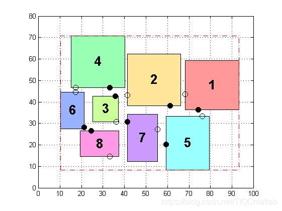
三、运行结果

四、matlab版本及参考文献

1 matlab版本
2014a

2 参考文献
[1] 包子阳,余继周,杨杉.智能优化算法及其MATLAB实例（第2版）[M].电子工业出版社，2016.
[2]张岩,吴水根.MATLAB优化算法源代码[M].清华大学出版社，2017.

文章来源: qq912100926.blog.csdn.net，作者：海神之光，版权归原作者所有，如需转载，请联系作者。

原文链接：qq912100926.blog.csdn.net/article/details/112684319