【物理应用】基于matlab PIC模型太阳风粒子模拟【含Matlab源码 493期】

一、获取代码方式

获取代码方式1：
通过订阅紫极神光博客付费专栏，凭支付凭证，私信博主，可获得此代码。

获取代码方式2：
完整代码已上传我的资源：【物理应用】基于matlab PIC模型太阳风粒子模拟【含Matlab源码 493期】

备注：
订阅紫极神光博客付费专栏，可免费获得1份代码（有效期为订阅日起，三天内有效）；

二、部分源代码

%%%%%%%%%%%%%%%%%%%%%%%%%%%%%%%%%%%%%%%%%%%%%%%%%%%%%%%%%%%%%%%%%%%
% Si
%
% For more, 
% and
%%%%%%%%%%%%%%%%%%%%%%%%%%%%%%%%%%%%%%%%%%%%%%%%%%%%%%%%%%%%%%%%%%%

%reset variables
clear variables

%identify globals needed by the potential solver
global EPS0 QE den A n0 phi0 phi_p Te box 

%setup constants
EPS0 = 8.854e-12;		%permittivity of free space
QE = 1.602e-19;			%elementary charge
K = 1.381e-23;			%boltzmann constant
AMU = 1.661e-27;		%atomic mass unit
M = 32*AMU;             %ion mass (molecular oxygen)

%input settings
n0 = 1e12;				%density in #/m^3
phi0 = 0;               %reference potential 
Te = 1;                 %electron temperature in eV
Ti = 0.1;              	%ion velocity in eV
v_drift = 7000;        	%ion injection velocity, 7km/s
phi_p = -5;            	%wall potential

%calculate plasma parameters
lD = sqrt(EPS0*Te/(n0*QE));    	%Debye length
vth = sqrt(2*QE*Ti/M);			%thermal velocity with Ti in eV

%set simulation domain
nx = 16;               %number of nodes in x direction
ny = 10;               %number of nodes in y direction
ts = 200;              %number of time steps
dh = lD;               %cell size
np_insert = (ny-1)*15; %insert 15 particles per cell

%compute some other values
nn = nx*ny;             %total number of nodes
dt = 0.1*dh/v_drift;	%time step, at vdrift move 0.10dx
Lx = (nx-1)*dh;         %domain length in x direction
Ly = (ny-1)*dh;         %domain length in y direction

%specify plate dimensions
box(1,:) = [floor(nx/3) floor(nx/3)+2]; %x range
box(2,:) = [1 floor(ny/2)];             %y range

%create an object domain for visualization
object = zeros(nx,ny);
for j=box(2,1):box(2,2)
    object(box(1,1):box(1,2),j)=ones(box(1,2)-box(1,1)+1,1);
end

%calculate specific weight
flux = n0*v_drift*Ly;       %flux of entering particles
npt = flux*dt;              %number of real particles created per timestep
spwt = npt/np_insert;       %specific weight, real particles per macroparticle
mp_q = 1;                   %macroparticle charge
max_part=20000;             %buffer size

%allocate particle array
part_x = zeros(max_part,2); %particle positions
part_v = zeros(max_part,2); %particle velocities

%set up multiplication matrix for potential solver
%here we are setting up the Finite Difference stencil

A = zeros(nn);              %allocate empty nn * nn matrix

%set regular stencil on internal nodes
for j=2:ny-1                    %only internal nodes
    for i=2:nx-1
        u = (j-1)*nx+i;         %unknown (row index)
        
        A(u,u) = -4/(dh*dh);    %phi(i,j)
        A(u,u-1)=1/(dh*dh);     %phi(i-1,j)
        A(u,u+1)=1/(dh*dh);     %phi(i+1,j)
        A(u,u-nx)=1/(dh*dh);    %phi(i,j-1)
        A(u,u+nx)=1/(dh*dh);    %phi(i,j+1)
    end  
end

%neumann boundary on y=0
for i=1:nx
    u=i;
    A(u,u) = -1/dh;              %phi(i,j)
    A(u,u+nx) = 1/dh;            %phi(i,j+1)
end

%neumann boundary on y=Ly
for i=1:nx
    u=(ny-1)*nx+i;
    A(u,u-nx) = 1/dh;            %phi(i,j-1)
    A(u,u) = -1/dh;              %phi(i,j)
end

%neumann boundary on x=Lx
for j=1:ny
    u=(j-1)*nx+nx;
    A(u,:)=zeros(1,nn);         %clear row
    A(u,u-1) = 1/dh;            %phi(i-1,j)
    A(u,u) = -1/dh;             %phi(i,j)
end

%dirichlet boundary on x=0
for j=1:ny
    u=(j-1)*nx+1;
    A(u,:)=zeros(1,nn);         %clear row
    A(u,u) = 1;                 %phi(i,j)
end

%dirichlet boundary on nodes corresponding to the plate
for j=box(2,1):box(2,2)
    for i=box(1,1):box(1,2)
        u=(j-1)*nx+i;
        A(u,:)=zeros(1,nn);     %clear row
        A(u,u)=1;               %phi(i,j)
    end
end

%initialize
phi = ones(nx,ny)*phi0;         %set initial potential to phi0
np = 0;                         %clear number of particles

disp(['Solving potential for the first time. Please be patient, this could take a while.']);

%%%%%%%%%%%%%%%%%%%%%%%%
% MAIN LOOP
%%%%%%%%%%%%%%%%%%%%%%%%
for it=1:ts                     %iterate for ts time steps
      	    
	%reset field quantities
	den = zeros(nx,ny);         %number density
	efx = zeros(nx,ny);         %electric field, x-component
    efy = zeros(nx,ny);         %electric field, y-component
	chg = zeros(nx,ny);         %charge distribution
    
    %*** 1. CALCULATE CHARGE DENSITY ***
	
    % deposit charge to nodes
	for p=1:np                          %loop over particles
		fi = 1+part_x(p,1)/dh;          %real i index of particle's cell
		i = floor(fi);                  %integral part
		hx = fi-i;                      %the remainder
        
        fj = 1+part_x(p,2)/dh;          %real j index of particle's cell
        j = floor(fj);                  %integral part
        hy = fj-j;                      %the remainder

        %interpolate charge to nodes
		chg(i,j) = chg(i,j) + (1-hx)*(1-hy);
		chg(i+1,j) = chg(i+1,j) + hx*(1-hy);
        chg(i,j+1) = chg(i,j+1) + (1-hx)*hy;
        chg(i+1,j+1) = chg(i+1,j+1) + hx*hy;
	end 

	%calculate density
	den = spwt*mp_q*chg/(dh*dh);
    
    %apply boundaries
	den(1,:) = 2*den(1,:);      %double density since only half volume contributing
    den(nx,:) = 2*den(nx,:);
    den(:,1) = 2*den(:,1);
    den(:,ny) = 2*den(:,ny);
    
    %add density floor for plotting and to help the solver
    den = den + 1e4;
	
	%*** 2. CALCULATE POTENTIAL ***    
    phi = eval_2dpot_GS(phi);
	
	%*** 3. CALCULATE ELECTRIC FIELD ***
	efx(2:nx-1,:) = phi(1:nx-2,:) - phi(3:nx,:);  %central difference on internal nodes
    efy(:,2:ny-1) = phi(:,1:ny-2) - phi(:,3:ny);  %central difference on internal nodes
    efx(1,:) = 2*(phi(1,:) - phi(2,:));           %forward difference on x=0
    efx(nx,:) = 2*(phi(nx-1,:) - phi(nx,:));      %backward difference on x=Lx
    efy(:,1) = 2*(phi(:,1) - phi(:,2));           %forward difference on y=0
    efy(:,ny) = 2*(phi(:,ny-1) - phi(:,ny));      %forward difference on y=Ly
    
    efx = efx / (2*dh);    %divide by dominator
    efy = efy / (2*dh);

    %*** 4. GENERATE NEW PARTICLE ***
    if (np+np_insert>=max_part)     %make sure we don't exceed array limits
  %      np_insert=max_part-np;
    end

    %insert particles randomly distributed in y and in the first cell
    part_x(np+1:np+np_insert,1)=rand(np_insert,1)*dh;   %x position
    part_x(np+1:np+np_insert,2)=rand(np_insert,1)*Ly;   %y position

    %sample Maxwellian in x and y, add drift velocity in x
    part_v(np+1:np+np_insert,1)=v_drift+(-1.5+rand(np_insert,1)+rand(np_insert,1)+rand(np_insert,1))*vth;
    part_v(np+1:np+np_insert,2)=0.5*(-1.5+rand(np_insert,1)+rand(np_insert,1)+rand(np_insert,1))*vth;
    np=np+np_insert;    %increment particle counter

    %*** 5. MOVE PARTICLES ***
	p=1;
    while(p<=np)                        %loop over particles
		fi = 1+part_x(p)/dh;            %i index of particle's cell
		i  = floor(fi);
		hx = fi-i;                      %fractional x position in cell
        
        fj = 1+part_x(p,2)/dh;          %j index of particle' cell
        j = floor(fj);
        hy = fj-j;                      %fractional y position in cell
        
        %gather electric field
        E=[0 0];
  		E = [efx(i,j) efy(i,j)]*(1-hx)*(1-hy);      %contribution from (i,j)
		E = E+ [efx(i+1,j) efy(i+1,j)]*hx*(1-hy);   %(i+1,j)
        E = E + [efx(i,j+1) efy(i+1,j)]*(1-hx)*hy;  %(i,j+1)
        E = E + [efx(i+1,j+1) efy(i+1,j+1)]*hx*hy;  %(i+1,j+1)
        
        %update velocity and position
        F = QE*E;                           %Lorentz force, F=qE
		a = F/M;                            %acceleration
		part_v(p,:) = part_v(p,:)+a*dt;     %update velocity
		part_x(p,:) = part_x(p,:)+part_v(p,:)*dt;   %update position

  

 

  
1
  
2
  
3
  
4
  
5
  
6
  
7
  
8
  
9
  
10
  
11
  
12
  
13
  
14
  
15
  
16
  
17
  
18
  
19
  
20
  
21
  
22
  
23
  
24
  
25
  
26
  
27
  
28
  
29
  
30
  
31
  
32
  
33
  
34
  
35
  
36
  
37
  
38
  
39
  
40
  
41
  
42
  
43
  
44
  
45
  
46
  
47
  
48
  
49
  
50
  
51
  
52
  
53
  
54
  
55
  
56
  
57
  
58
  
59
  
60
  
61
  
62
  
63
  
64
  
65
  
66
  
67
  
68
  
69
  
70
  
71
  
72
  
73
  
74
  
75
  
76
  
77
  
78
  
79
  
80
  
81
  
82
  
83
  
84
  
85
  
86
  
87
  
88
  
89
  
90
  
91
  
92
  
93
  
94
  
95
  
96
  
97
  
98
  
99
  
100
  
101
  
102
  
103
  
104
  
105
  
106
  
107
  
108
  
109
  
110
  
111
  
112
  
113
  
114
  
115
  
116
  
117
  
118
  
119
  
120
  
121
  
122
  
123
  
124
  
125
  
126
  
127
  
128
  
129
  
130
  
131
  
132
  
133
  
134
  
135
  
136
  
137
  
138
  
139
  
140
  
141
  
142
  
143
  
144
  
145
  
146
  
147
  
148
  
149
  
150
  
151
  
152
  
153
  
154
  
155
  
156
  
157
  
158
  
159
  
160
  
161
  
162
  
163
  
164
  
165
  
166
  
167
  
168
  
169
  
170
  
171
  
172
  
173
  
174
  
175
  
176
  
177
  
178
  
179
  
180
  
181
  
182
  
183
  
184
  
185
  
186
  
187
  
188
  
189
  
190
  
191
  
192
  
193
  
194
  
195
  
196
  
197
  
198
  
199
  
200
  
201
  
202
  
203
  
204
  
205
  
206
  
207
  
208
  
209
  
210
  
211
  
212
  
213
  
214
  
215
  
216
  
217
  
218
  
219
  
220
  
221
 

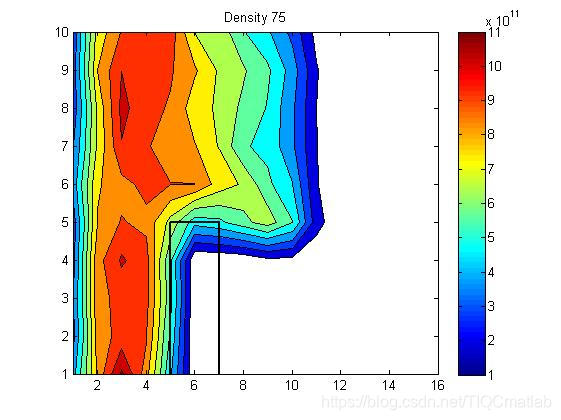
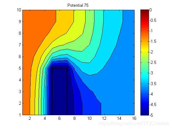
三、运行结果

四、matlab版本及参考文献

1 matlab版本
2014a

2 参考文献
[1] 门云阁.MATLAB物理计算与可视化[M].清华大学出版社，2013.

文章来源: qq912100926.blog.csdn.net，作者：海神之光，版权归原作者所有，如需转载，请联系作者。

原文链接：qq912100926.blog.csdn.net/article/details/114643928