【雷达通信】基于matlab无人机FMCW毫米波高度计雷达仿真【含Matlab源码 1261期】

一、获取代码方式

获取代码方式1：
完整代码已上传我的资源： 【雷达通信】基于matlab无人机FMCW毫米波高度计雷达仿真【含Matlab源码 1261期】

获取代码方式2：
通过订阅紫极神光博客付费专栏，凭支付凭证，私信博主，可获得此代码。

备注：订阅紫极神光博客付费专栏，可免费获得1份代码（有效期为订阅日起，三天内有效）；

二、FMCW毫米波简介

0 概念
FMCW(Frequency Modulated Continuous Wave)，即调频连续波。FMCW技术和脉冲雷达技术是两种在高精度雷达测距中使用的技术。其基本原理为发射波为高频连续波，其频率随时间按照三角波规律变化。
1 基础知识
FMCW雷达的核心是一种叫做线性调频脉冲的信号,线性调频脉冲是频率随时间以线性的方式增长的正弦波，在下图中

信号以fc的正弦波开始，然后他的频率不断增大，chirp信号的起始频率为 fc，带宽为B，信号的持续时间为Tc，则频率变化率（斜率）为:S=B/Tc

上图是简单的雷达示意图，有单个TX天线和单个RX天线，雷达工作过程大致为：1处的合成器生成一个线性调频脉冲，TX将脉冲传播出去，当脉冲遇到物体时会反射回来，RX接收反射的调频脉冲，TX和RX信号混在一起，最终在4处生成一种叫做IF（中频）的信号。下面详细了解以下关键元件4（混频器）。

混频器有两个输入一个输出，如果向混频器的两个输入端口输入两个正弦波，那么混频器将输出有以下两条性质的正弦波：
性质1：输出正弦波的瞬时频率等于两个输入正弦波的瞬时频率差值；
性质2：输出正弦波的起始相位等于两个输入正弦波的起始相位差值。

如上图， 被物体反射后的信号可以简单的看做是发射信号的延时，用t（时间差值）来表示，t=2d/c,接收信号与发射信号混频后的输出信号频率恒定，假设IF的频率为f,那么f=St=S2d/c (S为调频连续波的斜率)，其中d为物体的距离，c 为光速。对混频后的信号做FFT变换，可以得到单峰值频谱图。从上图中可以看出，为了避免产生距离判别模糊，t需要满足τ<Tc ，因此可得出系统所能探测的最远距离与Tc 有关。

三、部分源代码

%  
%  
% 1T1R Simulation. 
% Senario: UAV radar to horizontal ground/slope ground , height measurement.

clc;clear

%% Radar Parameters
fc = 24e9;   
c = physconst('LightSpeed');
lambda = c/fc;

tm = 5e-4;   % Chirp Cycle
bw = 300e6;    % FMCW Bandwidth
range_max = 5;     % Max detection Range 1~100 meters
v_max = 2.5;         % Max Velocity
%
range_res = c/2/bw;
sweep_slope = bw/tm;
fr_max = range2beat(range_max,sweep_slope,c);
fd_max = speed2dop(2*v_max,lambda);
fb_max = fr_max+fd_max;
fs = max(2*fb_max,bw);

%%
%% Use Phased Array System Toolbox to generate an FMCW waveform
waveform = phased.FMCWWaveform('SweepTime',tm,'SweepBandwidth',bw,...
'SampleRate',fs);
%%
tx_antenna = phased.IsotropicAntennaElement('FrequencyRange',[23.8e9 24.4e9],'BackBaffled',true);
rx_antenna = phased.IsotropicAntennaElement('FrequencyRange',[23.8e9 24.4e9],'BackBaffled',true);
%%
transmitter = phased.Transmitter('PeakPower',0.001,'Gain',20);
receiver = phased.ReceiverPreamp('Gain',20,'NoiseFigure',8.5,'SampleRate',fs);

txradiator = phased.Radiator('Sensor',tx_antenna,'OperatingFrequency',fc,...
'PropagationSpeed',c);
rxcollector = phased.Collector('Sensor',rx_antenna,'OperatingFrequency',fc,...
'PropagationSpeed',c);

rng(2020);
fs_d = 2500000;
Dn = fix(fs/fs_d);

%%
%% --------------Radar Motion Platform-------------- %%
radar_s = phased.Platform('InitialPosition',[0;0;0],...
    'Velocity',[0.05;2.3;-0.04]);  %% *********** Set Radar Velocity Here **************        

%% Targets ------------- Ground -------------------- %%
target_ypos = -6:0.15:6;
target_num = size(target_ypos,2);
target_xpos = 1.3*ones(1,target_num) + 0*1.1*target_ypos; %% *********** Set Ground Shape Here ************** 
target_zpos = zeros(1,target_num);

target_pos = [[target_xpos,target_xpos,target_xpos];
    [target_ypos,target_ypos,target_ypos];
    [target_zpos-0.15,target_zpos,target_zpos+0.155]];
target_num = target_num*3;

target_rcs = 0.02*ones(1,target_num);
targets_vel = [zeros(1,target_num);zeros(1,target_num);zeros(1,target_num)];

targets = phased.RadarTarget('MeanRCS',target_rcs,'PropagationSpeed',c,'OperatingFrequency',fc);
targetmotion = phased.Platform('InitialPosition',target_pos,...
    'Velocity',targets_vel);

%%
%% Signal Propogation
% simulation of free space propagtion
channel = phased.FreeSpace('PropagationSpeed',c,...
'OperatingFrequency',fc,'SampleRate',fs,'TwoWayPropagation',true);

%%
%%
% Generate Time Domain Waveforms of Chirps
% xr is the data received at rx array

Nsweep = 32;               % Number of Chirps (IF signal) of this simulation

chirp_len = fix(fs_d*waveform.SweepTime);
xr = complex(zeros(chirp_len,1,Nsweep));

disp('The simulation will take some time. Please wait...')
for m = 1:Nsweep
    if mod(m,1)==0
        disp([num2str(m),'/',num2str(Nsweep)])
    end
    
    % Update radar and target positions
    [radar_pos,radar_vel] = radar_s(waveform.SweepTime);
    [tgt_pos,tgt_vel] = targetmotion(waveform.SweepTime);
    [~,tgt_ang] = rangeangle(tgt_pos,radar_pos);
    
    % Transmit FMCW waveform
    sig = waveform();
    txsig = transmitter(sig);
    
    % Toggle transmit element
    txsig = txradiator(txsig,tgt_ang);
    
    % Propagate the signal and reflect off the target
    txsig = channel(txsig,radar_pos,tgt_pos,radar_vel,tgt_vel);
    txsig = targets(txsig);
    
    % Dechirp the received radar return
    rxsig = rxcollector(txsig,tgt_ang);
    rxsig = receiver(rxsig);
    dechirpsig = dechirp(rxsig,sig);
    
    % Decimate the return to reduce computation requirements
    for n = size(xr,2):-1:1
        xr(:,n,m) = decimate(dechirpsig(1:chirp_len*Dn,n),Dn,'FIR');
    end
end

range_res = range_res*size(dechirpsig,1)/Dn/size(xr,1);

%%
xrv = squeeze(xr);
save('vrv.mat',...
    'xrv','fc','fs_d','c','tm','bw','waveform','range_res',...
    'Nsweep','chirp_len','Dn','fb_max','lambda',...
    'v_max','range_max')

%%
%%
%%%%%%%%%%%%%%%%%%%%%%%%%%%%%%%%%%%%%%%%%%%%%%%%%%%%%
%         Part II: Signal Processing                %
%%%%%%%%%%%%%%%%%%%%%%%%%%%%%%%%%%%%%%%%%%%%%%%%%%%%%

%%
if ~exist('xrv')
    load('vrv.mat');
end
    
% FFT points
nfft_r = 2^nextpow2(size(xrv,1));
nfft_d = 2^nextpow2(size(xrv,2));
nfft_mul = 2;
ra_res = range_res*size(xrv,1)/nfft_mul/nfft_r;

% RDM Algorithm
rngdop = phased.RangeDopplerResponse('PropagationSpeed',c,...
    'DopplerOutput','Speed','OperatingFrequency',fc,'SampleRate',fs_d,...
    'RangeMethod','FFT','PRFSource','Property',...
    'RangeWindow','Hann','PRF',1/waveform.SweepTime,...
    'SweepSlope',waveform.SweepBandwidth/waveform.SweepTime,...
    'RangeFFTLengthSource','Property','RangeFFTLength',nfft_r*nfft_mul,...
    'DopplerFFTLengthSource','Property','DopplerFFTLength',nfft_d*nfft_mul,...
    'DopplerWindow','Hann');

% RD Map
[resp,r,sp] = rngdop(xrv);


% % Range-Energy Calibration
% for k=size(resp,1)/2+1:size(resp,1)
%     resp(k,:,:) = resp(k,:,:) * (k-size(resp,1)/2)^3;
% end

subplot(221);plotResponse(rngdop,squeeze(xrv));axis([-2*v_max 2*v_max 0 range_max-0.05])


%respmap = mag2db(abs(resp));
respmap = abs(resp);
respmap = avg_filter_2D(respmap,1);
subplot(222);mesh(respmap(nfft_r*nfft_mul/2+1:nfft_r*nfft_mul/2+1+30*nfft_mul,...
    :))
    %nfft_d*nfft_mul/2-12*nfft_mul:nfft_d*nfft_mul/2+12*nfft_mul))

subplot(413);plot(sum(respmap(nfft_r*nfft_mul/2+1:nfft_r*nfft_mul/2+1+30*nfft_mul,...
    nfft_d*nfft_mul/2-1:nfft_d*nfft_mul/2+2),2))



  

 

  
1
  
2
  
3
  
4
  
5
  
6
  
7
  
8
  
9
  
10
  
11
  
12
  
13
  
14
  
15
  
16
  
17
  
18
  
19
  
20
  
21
  
22
  
23
  
24
  
25
  
26
  
27
  
28
  
29
  
30
  
31
  
32
  
33
  
34
  
35
  
36
  
37
  
38
  
39
  
40
  
41
  
42
  
43
  
44
  
45
  
46
  
47
  
48
  
49
  
50
  
51
  
52
  
53
  
54
  
55
  
56
  
57
  
58
  
59
  
60
  
61
  
62
  
63
  
64
  
65
  
66
  
67
  
68
  
69
  
70
  
71
  
72
  
73
  
74
  
75
  
76
  
77
  
78
  
79
  
80
  
81
  
82
  
83
  
84
  
85
  
86
  
87
  
88
  
89
  
90
  
91
  
92
  
93
  
94
  
95
  
96
  
97
  
98
  
99
  
100
  
101
  
102
  
103
  
104
  
105
  
106
  
107
  
108
  
109
  
110
  
111
  
112
  
113
  
114
  
115
  
116
  
117
  
118
  
119
  
120
  
121
  
122
  
123
  
124
  
125
  
126
  
127
  
128
  
129
  
130
  
131
  
132
  
133
  
134
  
135
  
136
  
137
  
138
  
139
  
140
  
141
  
142
  
143
  
144
  
145
  
146
  
147
  
148
  
149
  
150
  
151
  
152
  
153
  
154
  
155
  
156
  
157
  
158
  
159
  
160
  
161
  
162
  
163
  
164
  
165
  
166
  
167
  
168
  
169
  
170
  
171
  
172
  
173
  
174
  
175
 

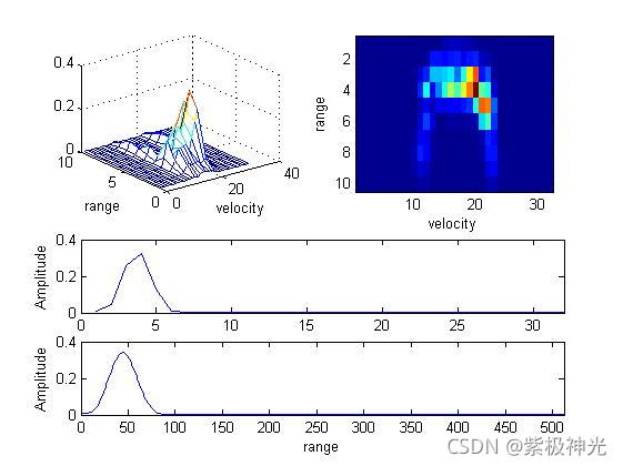
四、运行结果

五、matlab版本及参考文献

1 matlab版本
2014a

2 参考文献
[1] 沈再阳.精通MATLAB信号处理[M].清华大学出版社，2015.
[2]高宝建,彭进业,王琳,潘建寿.信号与系统——使用MATLAB分析与实现[M].清华大学出版社，2020.
[3]王文光,魏少明,任欣.信号处理与系统分析的MATLAB实现[M].电子工业出版社，2018.
[4]李树锋.基于完全互补序列的MIMO雷达与5G MIMO通信[M].清华大学出版社.2021
[5]何友,关键.雷达目标检测与恒虚警处理（第二版）[M].清华大学出版社.2011

文章来源: qq912100926.blog.csdn.net，作者：海神之光，版权归原作者所有，如需转载，请联系作者。

原文链接：qq912100926.blog.csdn.net/article/details/119951190