【印刷字符识别】基于matlab模板匹配英文字母识别【含Matlab源码 808期】

一、获取代码方式
获取代码方式1:
完整代码已上传我的资源: 【印刷字符识别】基于matlab模板匹配英文字母识别【含Matlab源码 808期】
获取代码方式2:
通过订阅紫极神光博客付费专栏,凭支付凭证,私信博主,可获得此代码。
备注:订阅紫极神光博客付费专栏,可免费获得1份代码(有效期为订阅日起,三天内有效);
二、简介
1 概述
模式识别就是通过计算机,用数学模型求解的方法研究模式的自动处理和判读。在模式识别的各种方法中,模板匹配是最容易的一种,其数学模型易于建立,通过模板匹配对数字图像模式识别有助于我们了解数学模型在数字图像中的应用。
2 模板匹配算法
2.1 相似性测度求匹配
模板匹配的实际操作思路很简单:拿已知的模板,和原图像中同样大小的一块区域去对。最开始时,模板的左上角点和图像的左上角点是重合的,拿模板和原图像中同样大小的一块区域去对比,然后平移到下一个像素,仍然进行同样的操作, ……所有的位置都对完后,差别最小的那块就是我们要找的物体。
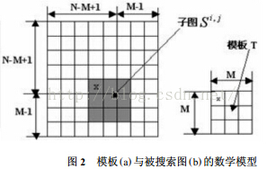
以上所描述的是相似性测度法求匹配的求解思路,其在计算机中操作的如图2所示。设模板T叠放在搜索图上平移,被模板覆盖搜索图下的那个图像叫做子图Si , j,i , j 为这块子图的左上角像素点在S图的坐标,称为参考点,从图2可知,i , j 的取值范围是:1<i ,j <N- M+1. 现在可以比较T和Si , j的内容。若两者一致,则T和S之差为零. 因此,可用下列公式(1) 和公式(2) 来衡量T和Si , j的相似程度。
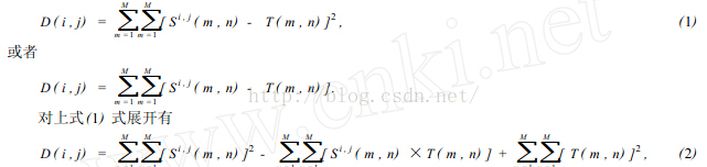
在(2) 式中第3项表示模板总能量,是一个与(i , j) 无关的常数;第1项是模板覆盖下子图的能量,它随着(i , j) 的位置缓慢地改变;第2项表示的子图与模板的互相关系,随着(i , j) 的改变而改变,当T和Si , j匹配时这项取值最大。因此可用下列相关函数(3) 作相似性测度。

当矢量t 和S1之间的夹角为0时,即当S1(i , j) =kt 时(k为常量) ,有R(i , j) =1,否则R(i , j) <1. 显然R(i , j) 越大,模板T和Si , j就越相似,点(i , j) 就是我们要寻找的匹配点。
2.2 序贯相似性检测的算法
用相关法求匹配的计算量很大,因为模板要在(N- M+1)2个参考位置上作相关计算,除了在匹配点外,其它点作的都是无用功。因此,人们提出一种叫序贯相似性检测的算法,简称SSDA(Sequential SimiliarityDetectionAlgorithm) 其要点是:
在数字图像中,SSDA法用公式(6) 计算图像f ( x, y) 在点(i , j) 的非相似度m(i , j) 作为匹配尺度。式中(i , j) 表示的不是模板中心坐标,而是它左上角坐标。模板的大小为n ×m。

如果在(i , j) 处图像中有和模板一致的图案时,则m(i , j) 值很小,反之则很大。特别是模板和搜索图下的子图部分,完全不一致的场合下,如果在模板内的各像素与图像重合部分对应的像素灰度差的绝对值依次增加,其和会急剧增大。 因此,在作加法时,如果灰度差的绝对值部分和超过某一阈值时,就认为这个位置不存在和模板一致的图案,从而转移到下一个位置上计算m(i , j)。并且在这模板下的各像素点计算中止,因此能大幅度地缩短计算时间,提高匹配速度。
根据上述思路,我们可以进一步改进SSDA算法。就是把在图像上的模板移动分为粗检索和细检索2个阶段进行。首先进行粗检索,它不是让模板每次移动1个像素,而是每隔若干的像素把模板和图像重叠,并且计算匹配的尺度,从而求出待寻找的图案大致存在的范围。然后在这个范围内,让模板每隔1个像素移动1次,根据匹配的尺度确定寻找图案的所在位置。这样,整体上计算模板匹配的次数减少了,计算时间缩短,匹配的速度提高了。但用这种方法具有漏掉图像中最恰当位置的危险性。
2.3 相关算法
2个函数的相关性定义,可用公式(7)表示:

f*表示f 的复共轭。我们知道相关理论类似卷积理论,F( u, v) 和 H( u, v) 分别表示f ( x, y) 和h( x, y)的傅立叶变换. 根据卷积理论有

可知卷积是空间域过滤和频率域过滤之间的纽带。相关的重要用途在于匹配。在匹配中,f ( x, y) 是一幅包含物体或区域的图像。如果想要确定f 是否包含有感兴趣的物体或区域,让h( x, y) 作为那个物体的区域(通常称该图像为模板)。如果匹配成功,2个函数的相关值会在h找到f 中相应点的位置上达到最大。从上面分析可知,相关算法可以有2种方法:可在空间域进行,也可在频率域进行。
2.4 幅度排序相关算法
这种算法有2个步骤组成:
第1步,把实时图中的各个灰度值按幅度的大小排成列的形式,然后在对它进行二进制(或三进制) 编码,根据二进制排序的序列,把实时图变换为二进制阵列的一个有序的集合{ Cn, n =1,2, …, N}。这一过程称之为幅度排序预处理。
第2步,序贯地将这些二进制序列与基准图进行由粗到细的相关,直到确定出匹配点为止。由于篇幅的限制,这里就不列出例子了。
2.5 分层搜索的序惯判决算法
这种分层搜索算法是直接基于人们先粗后细寻找事物的惯例而形成的,例如,在中国地图上找肇庆的位置时,可以先找广东省这个地域,这过程称为粗相关。然后在这个地域中,再仔细确定肇庆的位置,这叫做细相关。很明显,利用这种方法,可以很快找出肇庆的位置。因为在这过程中省略了寻找广东省以外区域所需的时间,这种方法称为分层搜索的序贯判决法,利用这种思想形成的分层算法具有相当高的搜索速度。限于篇幅,这里只给出这种操作的一般思路。
3 总结
模式匹配本质就是应用数学。模板匹配过程如下:①将图像数字化,按顺序取出每个点的像素值;②代入事先建立的数学模型进行预处理;③选择一种合适的算法进行模式匹配;④将匹配后图像的坐标列出或直接在原图显示.。在模板匹配操作中最为关键的是如何建立数学模型,这是正确匹配的核心。
三、部分源代码
function varargout = main(varargin)
% MAIN MATLAB code for main.fig
%      MAIN, by itself, creates a new MAIN or raises the existing
%      singleton*.
%
%      H = MAIN returns the handle to a new MAIN or the handle to
%      the existing singleton*.
%
%      MAIN('CALLBACK',hObject,eventData,handles,...) calls the local
%      function named CALLBACK in MAIN.M with the given input arguments.
%
%      MAIN('Property','Value',...) creates a new MAIN or raises the
%      existing singleton*.  Starting from the left, property value pairs are
%      applied to the GUI before main_OpeningFcn gets called.  An
%      unrecognized property name or invalid value makes property application
%      stop.  All inputs are passed to main_OpeningFcn via varargin.
%
%      *See GUI Options on GUIDE's Tools menu.  Choose "GUI allows only one
%      instance to run (singleton)".
%
% See also: GUIDE, GUIDATA, GUIHANDLES

% Edit the above text to modify the response to help main

% Last Modified by GUIDE v2.5 06-Mar-2020 08:13:36

% Begin initialization code - DO NOT EDIT
gui_Singleton = 1;
gui_State = struct('gui_Name',       mfilename, ...
                   'gui_Singleton',  gui_Singleton, ...
                   'gui_OpeningFcn', @main_OpeningFcn, ...
                   'gui_OutputFcn',  @main_OutputFcn, ...
                   'gui_LayoutFcn',  [] , ...
                   'gui_Callback',   []);
if nargin && ischar(varargin{1})
    gui_State.gui_Callback = str2func(varargin{1});
end

if nargout
    [varargout{1:nargout}] = gui_mainfcn(gui_State, varargin{:});
else
    gui_mainfcn(gui_State, varargin{:});
end
% End initialization code - DO NOT EDIT


% --- Executes just before main is made visible.
function main_OpeningFcn(hObject, eventdata, handles, varargin)
% This function has no output args, see OutputFcn.
% hObject    handle to figure
% eventdata  reserved - to be defined in a future version of MATLAB
% handles    structure with handles and user data (see GUIDATA)
% varargin   command line arguments to main (see VARARGIN)

% Choose default command line output for main
handles.output = hObject;

% Update handles structure
guidata(hObject, handles);

% UIWAIT makes main wait for user response (see UIRESUME)
% uiwait(handles.figure1);


% --- Outputs from this function are returned to the command line.
function varargout = main_OutputFcn(hObject, eventdata, handles)
% varargout  cell array for returning output args (see VARARGOUT);
% hObject    handle to figure
% eventdata  reserved - to be defined in a future version of MATLAB
% handles    structure with handles and user data (see GUIDATA)

% Get default command line output from handles structure
varargout{1} = handles.output;


% --- Executes on button press in pushbutton1.
function pushbutton1_Callback(hObject, eventdata, handles)
% hObject    handle to pushbutton1 (see GCBO)
% eventdata  reserved - to be defined in a future version of MATLAB
% handles    structure with handles and user data (see GUIDATA)
al=['a' 'b' 'c' 'd' 'e' 'f' 'g' 'h' 'i' 'j' 'k' 'l' 'm' 'n' 'o' 'p' 'q' 'r' 's' 't' 'u' 'v' 'w' 'x' 'y' 'z'];
[filename pathname] =uigetfile({'*.png';'*.*'},'打开图片');
str=[pathname filename];
if str(1)~=0
    I=imread(str);
    axes(handles.axes1);
    imshow(I);
    [alpha num]=Imagedeal(str);
    G=[];
    for kkkk=1:num
    % Solve an Input-Output Fitting problem with a Neural Network
% Script generated by Neural Fitting app
% Created 04-Dec-2018 12:32:56
%
% This script assumes these variables are defined:
%
%   Train_Data - input data.
%   Train_Result - target data.

x = Train_Data;
t = Train_Result;

% Choose a Training Function
% For a list of all training functions type: help nntrain
% 'trainlm' is usually fastest.
% 'trainbr' takes longer but may be better for challenging problems.
% 'trainscg' uses less memory. Suitable in low memory situations.
trainFcn = 'trainscg';  % Scaled conjugate gradient backpropagation.

% Create a Fitting Network
hiddenLayerSize = 113;
net = fitnet(hiddenLayerSize,trainFcn);

% Choose Input and Output Pre/Post-Processing Functions
% For a list of all processing functions type: help nnprocess
net.input.processFcns = {'removeconstantrows','mapminmax'};
net.output.processFcns = {'removeconstantrows','mapminmax'};

% Setup Division of Data for Training, Validation, Testing
% For a list of all data division functions type: help nndivide
net.divideFcn = 'dividerand';  % Divide data randomly
net.divideMode = 'sample';  % Divide up every sample
net.divideParam.trainRatio = 70/100;
net.divideParam.valRatio = 15/100;
net.divideParam.testRatio = 15/100;

% Choose a Performance Function
% For a list of all performance functions type: help nnperformance
net.performFcn = 'mse';  % Mean Squared Error

% Choose Plot Functions
% For a list of all plot functions type: help nnplot
net.plotFcns = {'plotperform','plottrainstate','ploterrhist', ...
    'plotregression', 'plotfit'};

% Train the Network
[net,tr] = train(net,x,t);

% Test the Network
y = net(x);
e = gsubtract(t,y);
performance = perform(net,t,y)

% Recalculate Training, Validation and Test Performance
trainTargets = t .* tr.trainMask{1};
valTargets = t .* tr.valMask{1};
testTargets = t .* tr.testMask{1};
trainPerformance = perform(net,trainTargets,y)
valPerformance = perform(net,valTargets,y)
testPerformance = perform(net,testTargets,y)

% View the Network
view(net)

% Plots
% Uncomment these lines to enable various plots.
%figure, plotperform(tr)
%figure, plottrainstate(tr)
%figure, ploterrhist(e)
%figure, plotregression(t,y)
%figure, plotfit(net,x,t)

% Deployment
% Change the (false) values to (true) to enable the following code blocks.
% See the help for each generation function for more information.
if (false)
    % Generate MATLAB function for neural network for application
    % deployment in MATLAB scripts or with MATLAB Compiler and Builder
    % tools, or simply to examine the calculations your trained neural
    % network performs.
    genFunction(net,'myNeuralNetworkFunction');
    y = myNeuralNetworkFunction(x);
end
if (false)
    % Generate a matrix-only MATLAB function for neural network code
    % generation with MATLAB Coder tools.
    genFunction(net,'myNeuralNetworkFunction','MatrixOnly','yes');
    y = myNeuralNetworkFunction(x);
end
if (false)
    % Generate a Simulink diagram for simulation or deployment with.
    % Simulink Coder tools.
    gensim(net);
end
- 1
- 2
- 3
- 4
- 5
- 6
- 7
- 8
- 9
- 10
- 11
- 12
- 13
- 14
- 15
- 16
- 17
- 18
- 19
- 20
- 21
- 22
- 23
- 24
- 25
- 26
- 27
- 28
- 29
- 30
- 31
- 32
- 33
- 34
- 35
- 36
- 37
- 38
- 39
- 40
- 41
- 42
- 43
- 44
- 45
- 46
- 47
- 48
- 49
- 50
- 51
- 52
- 53
- 54
- 55
- 56
- 57
- 58
- 59
- 60
- 61
- 62
- 63
- 64
- 65
- 66
- 67
- 68
- 69
- 70
- 71
- 72
- 73
- 74
- 75
- 76
- 77
- 78
- 79
- 80
- 81
- 82
- 83
- 84
- 85
- 86
- 87
- 88
- 89
- 90
- 91
- 92
- 93
- 94
- 95
- 96
- 97
- 98
- 99
- 100
- 101
- 102
- 103
- 104
- 105
- 106
- 107
- 108
- 109
- 110
- 111
- 112
- 113
- 114
- 115
- 116
- 117
- 118
- 119
- 120
- 121
- 122
- 123
- 124
- 125
- 126
- 127
- 128
- 129
- 130
- 131
- 132
- 133
- 134
- 135
- 136
- 137
- 138
- 139
- 140
- 141
- 142
- 143
- 144
- 145
- 146
- 147
- 148
- 149
- 150
- 151
- 152
- 153
- 154
- 155
- 156
- 157
- 158
- 159
- 160
- 161
- 162
- 163
- 164
- 165
- 166
- 167
- 168
- 169
- 170
- 171
- 172
- 173
- 174
- 175
- 176
- 177
- 178
- 179
- 180
- 181
- 182
- 183
- 184
四、运行结果


五、matlab版本及参考文献
1 matlab版本
2014a
2 参考文献
[1] 蔡利梅.MATLAB图像处理——理论、算法与实例分析[M].清华大学出版社,2020.
[2]杨丹,赵海滨,龙哲.MATLAB图像处理实例详解[M].清华大学出版社,2013.
[3]周品.MATLAB图像处理与图形用户界面设计[M].清华大学出版社,2013.
[4]刘成龙.精通MATLAB图像处理[M].清华大学出版社,2015.
文章来源: qq912100926.blog.csdn.net,作者:海神之光,版权归原作者所有,如需转载,请联系作者。
原文链接:qq912100926.blog.csdn.net/article/details/115982675

- 点赞
- 收藏
- 关注作者
评论(0)