【图像融合】基于matlab小波变换全聚焦图像融合【含Matlab源码 1372期】

一、获取代码方式
获取代码方式1:
通过订阅紫极神光博客付费专栏,凭支付凭证,私信博主,可获得此代码。
获取代码方式2:
完整代码已上传我的资源:【图像融合】基于matlab小波变换全聚焦图像融合【含Matlab源码 1372期】
备注:
订阅紫极神光博客付费专栏,可免费获得1份代码(有效期为订阅日起,三天内有效);
二、小波变换简介
1974年,法国工程师J.Morlet首先提出小波变换的概念,1986年著名数学家Y.Meyer偶然构造出一个真正的小波基,并与S.Mallat合作建立了构造小波基的多尺度分析之后,小波分析才开始蓬勃发展起来。小波分析的应用领域十分广泛,在数学方面,它已用于数值分析、构造快速数值方法、曲线曲面构造、微分方程求解、控制论等。在信号分析方面的滤波、去噪声、压缩、传递等。在图像处理方面的图像压缩、分类、识别与诊断,去噪声等。本章将着重阐述小波在图像中的应用分析。
1 小波变换原理
小波分析是一个比较难的分支,用户采用小波变换,可以实现图像压缩,振动信号的分解与重构等,因此在实际工程上应用较广泛。小波分析与Fourier变换相比,小波变换是空间域和频率域的局部变换,因而能有效地从信号中提取信息。小波变换通过伸缩和平移等基本运算,实现对信号的多尺度分解与重构,从而很大程度上解决了Fourier变换带来的很多难题。
小波分析作一个新的数学分支,它是泛函分析、Fourier分析、数值分析的完美结晶;小波分析也是一种“时间—尺度”分析和多分辨分析的新技术,它在信号分析、语音合成、图像压缩与识别、大气与海洋波分析等方面的研究,都有广泛的应用。
(1)小波分析用于信号与图像压缩。小波压缩的特点是压缩比高,压缩速度快,压缩后能保持信号与图像的特征不变,且在传递中能够抗干扰。基于小波分析的压缩方法很多,具体有小波压缩,小波包压缩,小波变换向量压缩等。
(2)小波也可以用于信号的滤波去噪、信号的时频分析、信噪分离与提取弱信号、求分形指数、信号的识别与诊断以及多尺度边缘检测等。
(3)小波分析在工程技术等方面的应用概括的包括计算机视觉、曲线设计、湍流、远程宇宙的研究与生物医学方面。
2 多尺度分析
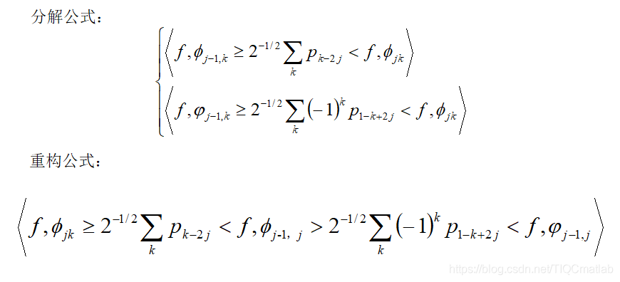
3 图像的分解和量化
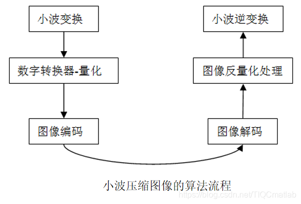
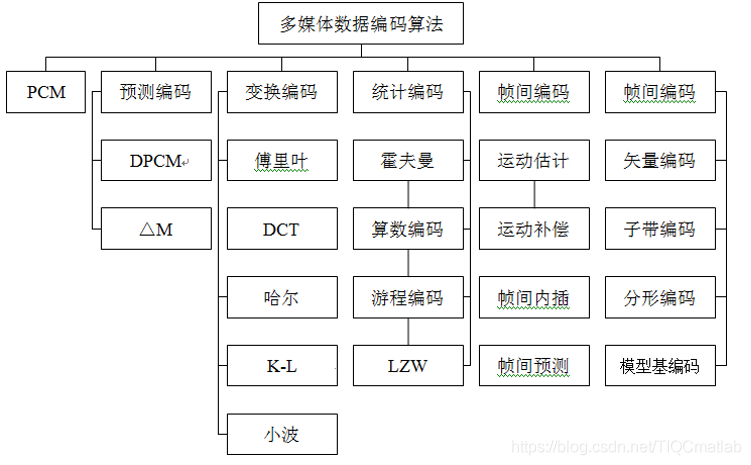
4 图像压缩编码
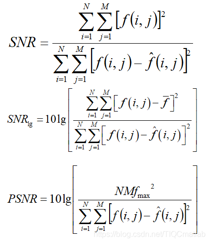
5 图像编码评价
三、部分源代码
clear all;
close all;
clc;
help imedgefuse;
%
% demo of deblurring
%
para.nLv = 5;
para.debug_mode = 1; % show message
para.wpropagation = 1; % weight propagation among subbands from parent to children
para.denoise = 1; % weight smoothing at each subbands for denoising
% J = imedgefuse( para, '001.jpg', '009.jpg', '016.jpg' );
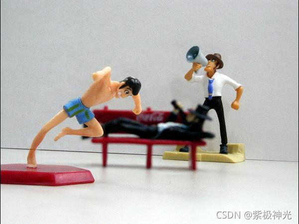
J = imedgefuse( para, '001.jpg', '016.jpg' );
figure( 1 ), imshow( J ); title( 'fused image' );
%
% demo of exposure fusion
%
para.nLv = 7;
para.debug_mode = 1;
para.wpropagation = 0; % weight propagation among subbands from parent to children
para.denoise = 1; % weight smoothing at each subbands for denoising
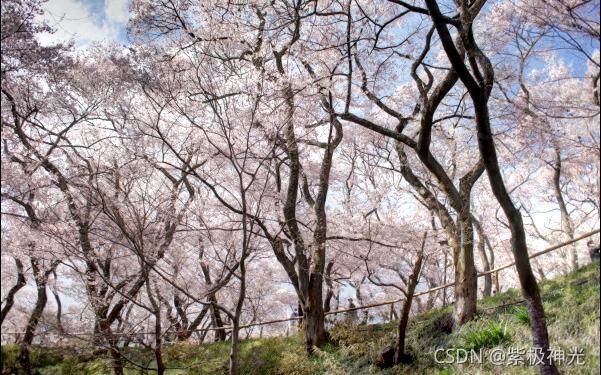
J = imedgefuse( para, 'takato_001.jpg', 'takato_002.jpg', 'takato_003.jpg' );
figure( 2 ), imshow( J ); title( 'fused image' );
function J = imedgefuse( para, varargin )
%IMEDGEFUSE composite images taken with different depth-of-fields
% as a result a pan focus image is generated.
%
% Usage:
%
% J = IMEDGEFUSE( para, fname, fname, ..., fname )
% J = IMEDGEFUSE( para, Image, Image, ..., Image )
%
% input arguments :
%
% para - parameters (the detail is described later)
% image - gray scale images (R^MxN) and rgb color images (R^MxNx3)
% fname - file names of input images
%
% output arguments :
%
% J - a fused image
%
% parameters :
%
% para.nLv = 6 - the total number of decompositions.
% para.propagate = 1 - weight propagation among subbands from parent to children.
% para.denoise = 1 - smoothing at each subbands for noise reduction.
% para.debug_mode = 1 - show debug message.
%
%
%
%
%
%
% parameters
%
global g_para;
set_parameters( para );
g_para.nImg = length( varargin ); % number of images
nImg = g_para.nImg;
nLv = g_para.nLv; % total number of decomposition
%
% Wavelet decomposition for the Y of YCbCr
%
DEBUG_MSG( 'Reading images and applying wavelet to them (Y of YCbCr)' );
for k = 1:nImg
% RGB color images are converted into the YCrCb color.
I = my_imread( varargin{ k } );
if k == 1 % initialization of the coefficient array
[ey, ex, nLv] = output_size( size(I,1), size(I,2), nLv );
C = zeros(ey,ex,nImg);
end
[C(:,:,k), S] = wavedec97( I(:,:,1), nLv );
DEBUG_MSG( '.' );
end
DEBUG_MSG( ' OK\n' );
W = gen3DWeightMatrix( C, S );
F = genNewSubbands( C, W );
J(:,:,1) = waverec97( F, S );
if g_para.bColor == 0
return
end
%
% Wavelet decomposition for the Cb of YCbCr
%
DEBUG_MSG( 'Reading pictures and applying wavelet to them (Cb of YCbCr)' );
for k = 1:nImg
I = my_imread( varargin{ k } );
[C(:,:,k), S] = wavedec97( I(:,:,2), nLv );
DEBUG_MSG( '.' );
end
DEBUG_MSG( ' OK\n' );
F = genNewSubbands( C, W );
J(:,:,2) = waverec97( F, S );
%
% Wavelet decomposition for the Cr of YCbCr
%
DEBUG_MSG( 'Reading pictures and applying wavelet to them (Cr of YCbCr)' );
for k = 1:nImg
I = my_imread( varargin{ k } );
[C(:,:,k), S] = wavedec97( I(:,:,3 ), nLv );
DEBUG_MSG( '.' );
end
DEBUG_MSG( ' OK\n' );
F = genNewSubbands( C, W );
J(:,:,3) = waverec97( F, S );
%
% Final conversion
%
J = ycbcr2rgb( J );
end
%
%--------------------------------------------------------------------------
%
function set_parameters( para )
global g_para;
g_para = para; % initialization
% total number of decompositions
if ~isfield( g_para, 'nLv' )
g_para.nLv = 5;
end
% weight propagation among subbands from parent to children
if ~isfield( g_para, 'propagate' )
g_para.propagate = 1;
end
% weight smoothing at each subband
if ~isfield( g_para, 'denoise' )
g_para.denoise = 1;
end
% hide debug message
if ~isfield( g_para, 'debug_mode' )
g_para.debug_mode = false(1);
end
g_para.bColor = true(1); % color image
end
- 1
- 2
- 3
- 4
- 5
- 6
- 7
- 8
- 9
- 10
- 11
- 12
- 13
- 14
- 15
- 16
- 17
- 18
- 19
- 20
- 21
- 22
- 23
- 24
- 25
- 26
- 27
- 28
- 29
- 30
- 31
- 32
- 33
- 34
- 35
- 36
- 37
- 38
- 39
- 40
- 41
- 42
- 43
- 44
- 45
- 46
- 47
- 48
- 49
- 50
- 51
- 52
- 53
- 54
- 55
- 56
- 57
- 58
- 59
- 60
- 61
- 62
- 63
- 64
- 65
- 66
- 67
- 68
- 69
- 70
- 71
- 72
- 73
- 74
- 75
- 76
- 77
- 78
- 79
- 80
- 81
- 82
- 83
- 84
- 85
- 86
- 87
- 88
- 89
- 90
- 91
- 92
- 93
- 94
- 95
- 96
- 97
- 98
- 99
- 100
- 101
- 102
- 103
- 104
- 105
- 106
- 107
- 108
- 109
- 110
- 111
- 112
- 113
- 114
- 115
- 116
- 117
- 118
- 119
- 120
- 121
- 122
- 123
- 124
- 125
- 126
- 127
- 128
- 129
- 130
- 131
- 132
- 133
- 134
- 135
- 136
- 137
- 138
- 139
- 140
- 141
- 142
- 143
- 144
- 145
- 146
- 147
- 148
- 149
- 150
- 151
- 152
- 153
- 154
- 155
- 156
- 157
- 158
- 159
- 160
- 161
- 162
- 163
- 164
- 165
- 166
- 167
- 168
- 169
- 170
- 171
- 172
- 173
- 174
- 175
- 176
四、运行结果
五、matlab版本及参考文献
1 matlab版本
2014a
2 参考文献
[1] 蔡利梅.MATLAB图像处理——理论、算法与实例分析[M].清华大学出版社,2020.
[2]杨丹,赵海滨,龙哲.MATLAB图像处理实例详解[M].清华大学出版社,2013.
[3]周品.MATLAB图像处理与图形用户界面设计[M].清华大学出版社,2013.
[4]刘成龙.精通MATLAB图像处理[M].清华大学出版社,2015.
文章来源: qq912100926.blog.csdn.net,作者:海神之光,版权归原作者所有,如需转载,请联系作者。
原文链接:qq912100926.blog.csdn.net/article/details/120635528

- 点赞
- 收藏
- 关注作者
评论(0)