【图像分割】基于matlab C-V模型水平集图像分割【含Matlab源码 1456期】

一、获取代码方式

获取代码方式1：
通过订阅紫极神光博客付费专栏，凭支付凭证，私信博主，可获得此代码。

获取代码方式2：
完整代码已上传我的资源：【图像分割】基于matlab C-V模型水平集图像分割【含Matlab源码 1456期】

备注：
订阅紫极神光博客付费专栏，可免费获得1份代码（有效期为订阅日起，三天内有效）；

二、图像分割简介

理论知识参考：【基础教程】基于matlab图像处理图像分割【含Matlab源码 191期】

三、部分源代码

%   Matlad code implementing Chan-Vese model in the paper 'Active Contours Without Edges'
%  
clear all;
close all;
Img=imread('Head.bmp');   
% Img=imread('vessel3.bmp'); % Note: this an example of images with intensity inhomogeneity. 
                             % CV model does not work for this image. 
Img=double(Img(:,:,1));

% get the size
[nrow,ncol] =size(Img);

ic=nrow/2;
jc=ncol/2;
r=10;  %起始园半径
initialLSF = sdf2circle(nrow,ncol,ic,jc,r);
u=initialLSF;


numIter = 200;
timestep = 0.5;
lambda_1=1;
lambda_2=1;
% h = 1;
h = 1;
epsilon=1;
nu = 0.001*255*255;  % tune this parameter for different images

% figure;
% imagesc(Img,[0 255]);colormap(gray)
% hold on;
% contour(u,[0 0],'r');


% start level set evolution
% for k=1:numIter
%     u=EVOL_CV(Img, u, nu, lambda_1, lambda_2, timestep, epsilon, 1);   % update level set function
%     if mod(k,10)==0
%         pause(.1);
%         imagesc(Img,[0 255]);colormap(gray)
%         hold on;
%         contour(u,[0 0],'r');
%         hold off;
%     end    
% end;

% start level set evolution
% figure;
% imagesc(Img, [0, 255]);colormap(gray);hold on;
% contour(u,[0 0],'r');                          
% title('Initial contour');   

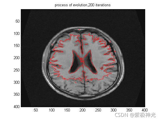
for k=1:numIter
    u=EVOL_CV(Img, u, nu, lambda_1, lambda_2, timestep, epsilon, 1);   % update level set function
    if mod(k,10)==0
        pause(.1);
        imagesc(Img,[0 255]);colormap(gray)
         hold on;
        contour(u,[0 0],'r'); 
        iterNum=[num2str(k), ' iterations'];        
        title(['process of evolution,',iterNum]);
        hold off;
    end    
end;

figure;
imagesc(Img, [0, 255]);colormap(gray);hold on;
contour(u,[0 0],'r'); 
totalIterNum=[num2str(k), ' iterations'];  
title(['Final contour, ', totalIterNum]);
function [C1,C2]= binaryfit(Img,H_phi) 
%   [C1,C2]= binaryfit(phi,U,epsilon) computes c1 c2 for optimal binary fitting 
%   input: 
%       Img: input image
%       phi: level set function
%       epsilon: parameter for computing smooth Heaviside and dirac function
%   output: 
%       C1: a constant to fit the image U in the region phi>0
%       C2: a constant to fit the image U in the region phi<0
%  
%   Author: Chunming Li, all right reserved
%   email: li_chunming@hotmail.com
%   URL:   http://www.engr.uconn.edu/~cmli/research/

a= H_phi.*Img;
numer_1=sum(a(:)); 
denom_1=sum(H_phi(:));
C1 = numer_1/denom_1;

b=(1-H_phi).*Img;
numer_2=sum(b(:));
c=1-H_phi;
denom_2=sum(c(:));
C2 = numer_2/denom_2;
function f = sdf2circle(nrow,ncol, ic,jc,r)
%   sdf2circle(nrow,ncol, ic,jc,r) computes the signed distance to a circle
%   input: 
%       nrow: number of rows
%       ncol: number of columns
%       (ic,jc): center of the circle
%       r: radius of the circle
%   output: 
%       f: signed distance to the circle
%  
%   created on 04/26/2004
%   author: Chunming Li
%   email: li_chunming@hotmail.com
%   Copyright (c) 2004-2006 by Chunming Li


[X,Y] = meshgrid(1:ncol, 1:nrow);

f = sqrt((X-jc).^2+(Y-ic).^2)-r;

%f=sdf2circle(100,50,51,25,10);figure;imagesc(f)



  

 

  
1
  
2
  
3
  
4
  
5
  
6
  
7
  
8
  
9
  
10
  
11
  
12
  
13
  
14
  
15
  
16
  
17
  
18
  
19
  
20
  
21
  
22
  
23
  
24
  
25
  
26
  
27
  
28
  
29
  
30
  
31
  
32
  
33
  
34
  
35
  
36
  
37
  
38
  
39
  
40
  
41
  
42
  
43
  
44
  
45
  
46
  
47
  
48
  
49
  
50
  
51
  
52
  
53
  
54
  
55
  
56
  
57
  
58
  
59
  
60
  
61
  
62
  
63
  
64
  
65
  
66
  
67
  
68
  
69
  
70
  
71
  
72
  
73
  
74
  
75
  
76
  
77
  
78
  
79
  
80
  
81
  
82
  
83
  
84
  
85
  
86
  
87
  
88
  
89
  
90
  
91
  
92
  
93
  
94
  
95
  
96
  
97
  
98
  
99
  
100
  
101
  
102
  
103
  
104
  
105
  
106
  
107
  
108
  
109
  
110
  
111
  
112
  
113
  
114
  
115
  
116
  
117
 

四、运行结果

五、matlab版本及参考文献

1 matlab版本
2014a

2 参考文献
[1] 蔡利梅.MATLAB图像处理——理论、算法与实例分析[M].清华大学出版社，2020.
[2]杨丹,赵海滨,龙哲.MATLAB图像处理实例详解[M].清华大学出版社，2013.
[3]周品.MATLAB图像处理与图形用户界面设计[M].清华大学出版社，2013.
[4]刘成龙.精通MATLAB图像处理[M].清华大学出版社，2015.
[5]赵勇,方宗德,庞辉,王侃伟.基于量子粒子群优化算法的最小交叉熵多阈值图像分割[J].计算机应用研究. 2008,(04)

文章来源: qq912100926.blog.csdn.net，作者：海神之光，版权归原作者所有，如需转载，请联系作者。

原文链接：qq912100926.blog.csdn.net/article/details/121087512