【图像配准】基于matlab OpenSUFT图像配准【含Matlab源码 1232期】

一、获取代码方式
获取代码方式1:
完整代码已上传我的资源:【图像配准】基于matlab OpenSUFT图像配准【含Matlab源码 1232期】
获取代码方式2:
通过订阅紫极神光博客付费专栏,凭支付凭证,私信博主,可获得此代码。
备注:
订阅紫极神光博客付费专栏,可免费获得1份代码(有效期为订阅日起,三天内有效);
二、SUFT配准简介
0 引言
目前, 红外检测技术广泛应用于电气设备和电路板卡的故障检测。图像配准技术是红外图像处理中最关键的技术之一, 配准的结果直接影响到故障的检测与定位。图像配准可分为基于灰度的图像配准和基于特征的图像配准。基于灰度的图像配准一般要求图像的相关性强, 而且计算量大, 很难达到实时性的需求;基于特征的图像配准计算量小、运算速度快, 且具有较强的鲁棒性, 成为图像配准研究的主要方向。
常用的特征提取算法有Harris, SUSAN, SIFT (Scale Invariant Features Transform) 和SUFT(Speeded-Up Robust Features) 等。SIFT算子最早由Lowe David G提出, 是建立在DoG (Difference of Gaussian) 尺度空间理论基础上的一种算法。该算法采取邻域方向性信息联合的思想, 从空间域和尺度域两个方面对图像进行特征分析, 对检测到的关键点用128维的特征向量表征, 具有尺度不变性和较强的鲁棒性。由对比分析知, SIFT算法性能优于Harris、SUSAN等角点算法, 但SIFT算子比较耗时, 不能满足实时性的要求。因此, Bay等人提出了一种基于快速鲁棒特征的SUFT算法, 它在特征点检测的准确性、鲁棒性以及实时性方面较其他算法有很大优势。
本文利用SUFT算法进行特征点检测, 采取粗匹配与精匹配结合的匹配策略选取特征点对, 设计了一种快速、有效、高精度的红外图像配准算法。
1 特征点提取
1.1 尺度空间特征点检测
SUFT特征点检测是基于Hessian矩阵进行的, 给定图像I (x, y) 中一点s=[x, y], 则在尺度σ的Hessian矩阵为

式中, Lxx (x, σ) 为图像I (x, y) 和高斯函数G (x, y, σ) 在x方向上的二阶导数在x的卷积。即

Lxy (x, σ) 、Lyy (x, σ) 与之类似。
高斯函数对尺度空间分析是最优的, 盒滤波器可近似为高斯函数二阶导数, 由式 (2) 易知SUFT算法可用盒滤波器近似Hessian矩阵。为了计算方便, 采用盒滤波器与输入图像的卷积Dxx 、Dyy 、Dxy 代替Lxx 、Lyy 、Lxy 。把9×9的盒滤波器近似为σ=1.2的二阶高斯导数Dxx、 Dxy与Lxx、Lxy之间关系为
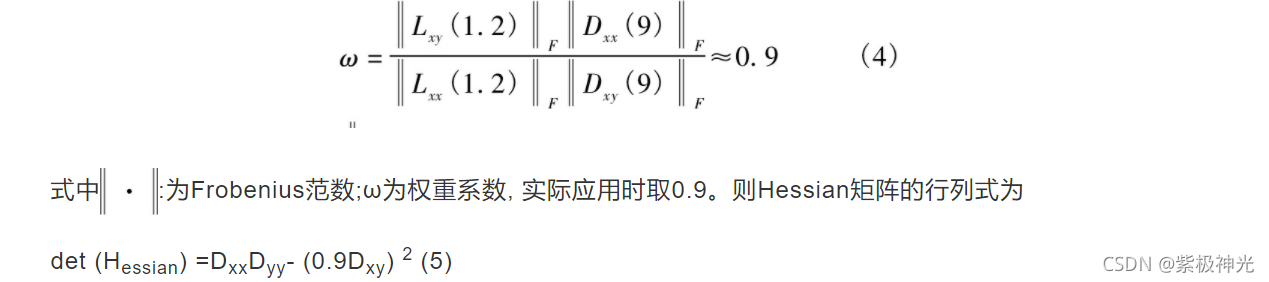
使用了盒滤波器和积分图像, 不必迭代地应用相同滤波器到前一个已滤层的输出上, 而是应用不同大小的盒滤波器以相同的速度直接作用到原始图像上, 见图1。

图1 尺度空间的金字塔示意图
因此, 对尺度空间的分析是通过增大滤波器的尺寸而不是迭代地降低图像的尺寸, 所需的计算时间是独立于滤波器尺寸的, 从而大大降低了运算时间。
1.2 特征点描述子的生成
为保证特征点旋转不变性, 要确定特征点主方向并建立坐标。以特征点为中心, 计算半径为6s (s为特征点所在尺度值) 邻域内的点在x、y方向的哈尔小波响应, 响应可表示为水平响应和垂直响应矢量和。按距离赋予响应值不同的高斯权重系数, 远离特征点的响应贡献小, 靠近特征点的响应贡献大。通过计算π/3滑动方向窗口内所有响应的和来估计主方向, 窗口内的水平响应和垂直响应分别被求和。两个响应的和产生一个局部方向向量, 定义窗口中最长的向量为特征点的主方向。
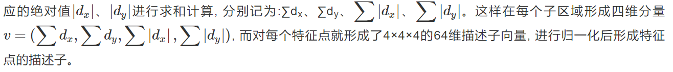
选定特征点主方向后, 以特征点为中心, 将坐标轴旋转到主方向上。选取周围边长为20s×20s的正方形区域, 并将该区域划分为4×4共16个子区域。在子区域内计算每个像素点x方向和y方向的哈尔小波响应, 记为dx、dy, 为了增强特征点描述子对几何变换及局部误差的鲁棒性, 可对dx、dy进行高斯权重系数赋值。然后对每个子区域的dx、dy响应以及响
2 图像配准方法及流程
利用SUFT算法提取红外图像中的特征点并生成特征点描述子, 采取欧氏距离最近邻粗匹配和相似四边形精匹配的方式提高配准精度, 然后使用8参数的平面透视变换模型描述匹配图像序列间的相对变换关系, 依据精匹配得到的匹配点对求解模型变换参数, 从而实现红外图像的配准。算法流程如图2所示。
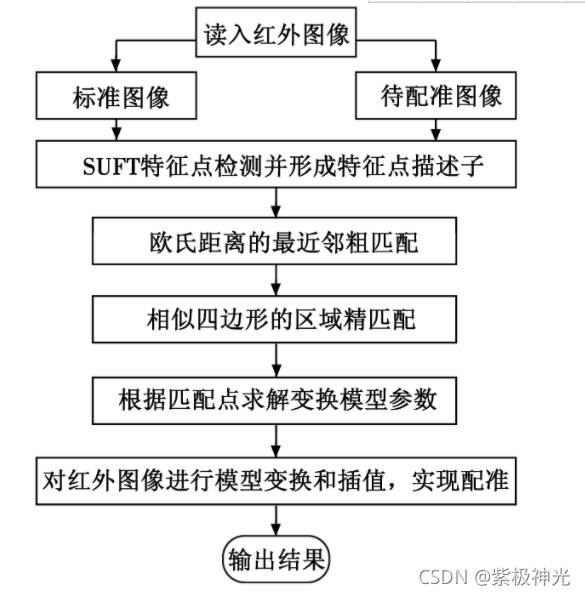
图2 本文算法流程图
算法具体实现过程如下。
-
利用SUFT算法分别检测标准图像F与待配准图像F′的特征点, 形成64维的特征点描述子。
-
最近邻匹配。以欧氏距离作为两个特征点描述子的相似性度量进行粗匹配, 算式为

式中:Xik表示图像F中第i个特征点对应特征向量的第k个元素;Xjk表示图像F′中第j个特征点对应特征向量的第k个元素;n为特征向量的维数。计算每个特征点对应特征向量的欧氏距离, 按照从小到大的顺序排列形成距离集合。设定阈值T1, 当特征点最小欧氏距离与次小欧氏距离的比值小于T1时, 认为这两个特征点匹配。T1越小, 匹配点对数目越少, 但更加稳定。 -
特征点精匹配。利用景物几何结构间的相似性, 在粗匹配点对中寻找相似四边形进行精匹配, 从而减少误匹配的概率。选取粗匹配点对中的一对匹配点作为四边形的一个固定顶点, 在粗匹配点对中随机选取三对匹配点组成两对四边形。由相似四边形性质可知, 若两四边形相似, 则对应四条边和两条对角线互成比例, 即满足
依据四边形相似的性质构造归一化的均方误差表达式e, 设定阈值T2 , 当e小于T2时认为两四边形相似。T2越小, 匹配精度越高, 由于SUFT提取特征点时存在误差, 故阈值不能设定太小, 通常设定比计算精度高出2~3个数量级, 本文T2设为0.05,
由图像F和F′中固定顶点组成相似四边形的数量判断是否为匹配点对, 剔除粗匹配点对中不能组成相似形的点对, 从而实现精匹配。 -
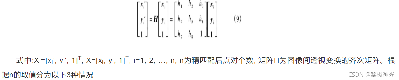
求解变换模型参数。由于红外热像仪拍摄位置的不固定性, 采用更加符合实际情况的8参数平面透视变换模型, 则图像F和F′对应像素点的关系为:X′=HX, 表示为
① 当n<4时, 适度增大阈值T1、T2, 重复步骤2) 、3) 以获得更多的精匹配点对;
② 当n=4时, 依据式 (9) 求解矩阵H;
③ 当n>4时, 属于过约束的情况, 利用最小二乘法求解H, 寻找一个最佳解使得每对匹配点的平面透视模型均方误差最小, 达到多个配准点拟合最优参数解的目的。 -
利用矩阵H对红外图像进行模型变换, 并通过线性插值得到变换后的图像, 从而实现图像配准。


三、部分源代码
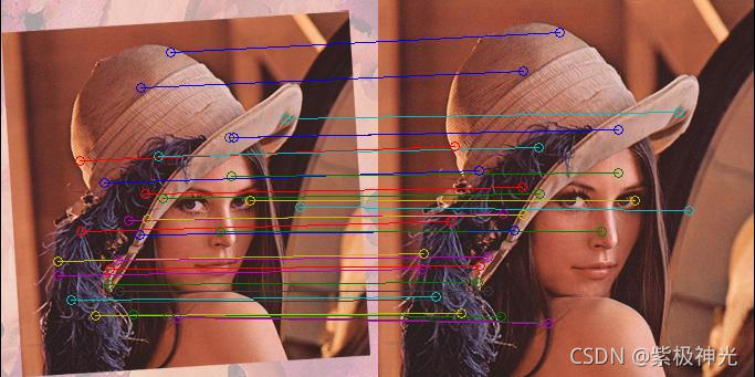
% Example 3, Affine registration
% Load images
I1=im2double(imread('TestImages/lena1.png'));
I2=im2double(imread('TestImages/lena2.png'));
% Get the Key Points
Options.upright=true;
Options.tresh=0.0001;
Ipts1=OpenSurf(I1,Options);
Ipts2=OpenSurf(I2,Options);
% Put the landmark descriptors in a matrix
D1 = reshape([Ipts1.descriptor],64,[]);
D2 = reshape([Ipts2.descriptor],64,[]);
% Find the best matches
err=zeros(1,length(Ipts1));
cor1=1:length(Ipts1);
cor2=zeros(1,length(Ipts1));
for i=1:length(Ipts1),
distance=sum((D2-repmat(D1(:,i),[1 length(Ipts2)])).^2,1);
[err(i),cor2(i)]=min(distance);
end
% Sort matches on vector distance
[err, ind]=sort(err);
cor1=cor1(ind);
cor2=cor2(ind);
% Make vectors with the coordinates of the best matches
Pos1=[[Ipts1(cor1).y]',[Ipts1(cor1).x]'];
Pos2=[[Ipts2(cor2).y]',[Ipts2(cor2).x]'];
Pos1=Pos1(1:30,:);
Pos2=Pos2(1:30,:);
% Show both images
I = zeros([size(I1,1) size(I1,2)*2 size(I1,3)]);
I(:,1:size(I1,2),:)=I1; I(:,size(I1,2)+1:size(I1,2)+size(I2,2),:)=I2;
figure, imshow(I); hold on;
% Show the best matches
plot([Pos1(:,2) Pos2(:,2)+size(I1,2)]',[Pos1(:,1) Pos2(:,1)]','-');
plot([Pos1(:,2) Pos2(:,2)+size(I1,2)]',[Pos1(:,1) Pos2(:,1)]','o');
% Calculate affine matrix
Pos1(:,3)=1; Pos2(:,3)=1;
M=Pos1'/Pos2';
% Add subfunctions to Matlab Search path
functionname='OpenSurf.m';
functiondir=which(functionname);
functiondir=functiondir(1:end-length(functionname));
addpath([functiondir '/WarpFunctions'])
% Warp the image
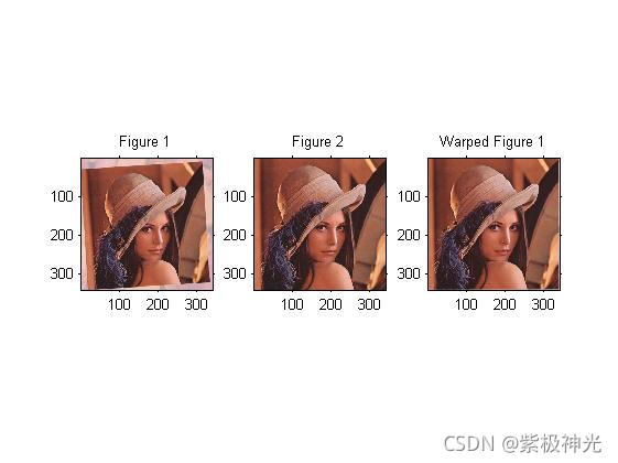
I1_warped=affine_warp(I1,M,'bicubic');
% Show the result
figure,
subplot(1,3,1), imshow(I1);title('Figure 1');
subplot(1,3,2), imshow(I2);title('Figure 2');
subplot(1,3,3), imshow(I1_warped);title('Warped Figure 1');
function [ipts, np]=FastHessian_interpolateExtremum(r, c, t, m, b, ipts, np)
% This function FastHessian_interpolateExtremum will ..
%
% [ipts,np] = FastHessian_interpolateExtremum( r,c,t,m,b,ipts,np )
%
% inputs,
% r :
% c :
% t :
% m :
% b :
% ipts :
% np :
%
% outputs,
% ipts :
% np :
%
% Function is written by D.Kroon University of Twente (July 2010)
D = FastHessian_BuildDerivative(r, c, t, m, b);
H = FastHessian_BuildHessian(r, c, t, m, b);
%get the offsets from the interpolation
Of = - H\D;
O=[ Of(1, 1), Of(2, 1), Of(3, 1) ];
%get the step distance between filters
filterStep = fix((m.filter - b.filter));
%If point is sufficiently close to the actual extremum
if (abs(O(1)) < 0.5 && abs(O(2)) < 0.5 && abs(O(3)) < 0.5)
np=np+1;
ipts(np).x = double(((c + O(1))) * t.step);
ipts(np).y = double(((r + O(2))) * t.step);
ipts(np).scale = double(((2/15) * (m.filter + O(3) * filterStep)));
ipts(np).laplacian = fix(FastHessian_getLaplacian(m,r,c,t));
end
function D=FastHessian_BuildDerivative(r,c,t,m,b)
dx = (FastHessian_getResponse(m,r, c + 1, t) - FastHessian_getResponse(m,r, c - 1, t)) / 2;
dy = (FastHessian_getResponse(m,r + 1, c, t) - FastHessian_getResponse(m,r - 1, c, t)) / 2;
ds = (FastHessian_getResponse(t,r, c) - FastHessian_getResponse(b,r, c, t)) / 2;
D = [dx;dy;ds];
function H=FastHessian_BuildHessian(r, c, t, m, b)
v = FastHessian_getResponse(m, r, c, t);
dxx = FastHessian_getResponse(m,r, c + 1, t) + FastHessian_getResponse(m,r, c - 1, t) - 2 * v;
dyy = FastHessian_getResponse(m,r + 1, c, t) + FastHessian_getResponse(m,r - 1, c, t) - 2 * v;
dss = FastHessian_getResponse(t,r, c) + FastHessian_getResponse(b,r, c, t) - 2 * v;
dxy = (FastHessian_getResponse(m,r + 1, c + 1, t) - FastHessian_getResponse(m,r + 1, c - 1, t) - FastHessian_getResponse(m,r - 1, c + 1, t) + FastHessian_getResponse(m,r - 1, c - 1, t)) / 4;
dxs = (FastHessian_getResponse(t,r, c + 1) - FastHessian_getResponse(t,r, c - 1) - FastHessian_getResponse(b,r, c + 1, t) + FastHessian_getResponse(b,r, c - 1, t)) / 4;
dys = (FastHessian_getResponse(t,r + 1, c) - FastHessian_getResponse(t,r - 1, c) - FastHessian_getResponse(b,r + 1, c, t) + FastHessian_getResponse(b,r - 1, c, t)) / 4;
H = zeros(3,3);
H(1, 1) = dxx;
H(1, 2) = dxy;
H(1, 3) = dxs;
H(2, 1) = dxy;
H(2, 2) = dyy;
H(2, 3) = dys;
H(3, 1) = dxs;
H(3, 2) = dys;
H(3, 3) = dss;
function descriptor=SurfDescriptor_GetDescriptor(ip, bUpright, bExtended, img, verbose)
% This function SurfDescriptor_GetDescriptor will ..
%
% [descriptor] = SurfDescriptor_GetDescriptor( ip,bUpright,bExtended,img )
%
% inputs,
% ip : Interest Point (x,y,scale, orientation)
% bUpright : If true not rotation invariant descriptor
% bExtended : If true make a 128 values descriptor
% img : Integral image
% verbose : If true show additional information
%
% outputs,
% descriptor : Descriptor of interest point length 64 or 128 (extended)
%
% Function is written by D.Kroon University of Twente (July 2010)
% Get rounded InterestPoint data
X = round(ip.x);
Y = round(ip.y);
S = round(ip.scale);
if (bUpright)
co = 1;
si = 0;
else
co = cos(ip.orientation);
si = sin(ip.orientation);
end
% Basis coordinates of samples, if coordinate 0,0, and scale 1
[lb,kb]=ndgrid(-4:4,-4:4); lb=lb(:); kb=kb(:);
%Calculate descriptor for this interest point
[jl,il]=ndgrid(0:3,0:3); il=il(:)'; jl=jl(:)';
ix = (il*5-8);
jx = (jl*5-8);
% 2D matrices instead of double for-loops, il, jl
cx=length(lb); cy=length(ix);
lb=repmat(lb,[1 cy]); lb=lb(:);
kb=repmat(kb,[1 cy]); kb=kb(:);
ix=repmat(ix,[cx 1]); ix=ix(:);
jx=repmat(jx,[cx 1]); jx=jx(:);
% Coordinates of samples (not rotated)
l=lb+jx; k=kb+ix;
%Get coords of sample point on the rotated axis
sample_x = round(X + (-l * S * si + k * S * co));
sample_y = round(Y + (l * S * co + k * S * si));
%Get the gaussian weighted x and y responses
xs = round(X + (-(jx+1) * S * si + (ix+1) * S * co));
ys = round(Y + ((jx+1) * S * co + (ix+1) * S * si));
gauss_s1 = SurfDescriptor_Gaussian(xs - sample_x, ys - sample_y, 2.5 * S);
rx = IntegralImage_HaarX(sample_y, sample_x, 2 * S,img);
ry = IntegralImage_HaarY(sample_y, sample_x, 2 * S,img);
%Get the gaussian weighted x and y responses on the aligned axis
rrx = gauss_s1 .* (-rx * si + ry * co); rrx=reshape(rrx,cx,cy);
rry = gauss_s1 .* ( rx * co + ry * si); rry=reshape(rry,cx,cy);
% Get the gaussian scaling
cx = -0.5 + il + 1; cy = -0.5 + jl + 1;
gauss_s2 = SurfDescriptor_Gaussian(cx - 2, cy - 2, 1.5);
if (bExtended)
% split x responses for different signs of y
check=rry >= 0; rrx_p=rrx.*check; rrx_n=rrx.*(~check);
dx = sum(rrx_p); mdx = sum(abs(rrx_p),1);
dx_yn = sum(rrx_n); mdx_yn = sum(abs(rrx_n),1);
% split y responses for different signs of x
check=(rrx >= 0); rry_p=rry.*check; rry_n=rry.*(~check);
dy = sum(rry_p,1);
mdy = sum(abs(rry_p),1);
dy_xn = sum(rry_n,1);
mdy_xn = sum(abs(rry_n),1);
else
dx = sum(rrx,1);
dy = sum(rry,1);
mdx = sum(abs(rrx),1);
mdy = sum(abs(rry),1);
dx_yn = 0; mdx_yn = 0;
dy_xn = 0; mdy_xn = 0;
end
if (bExtended)
descriptor=[dx;dy;mdx;mdy;dx_yn;dy_xn;mdx_yn;mdy_xn].* repmat(gauss_s2,[8 1]);
else
descriptor=[dx;dy;mdx;mdy].* repmat(gauss_s2,[4 1]);
end
len = sum((dx.^2 + dy.^2 + mdx.^2 + mdy.^2 + dx_yn + dy_xn + mdx_yn + mdy_xn) .* gauss_s2.^2);
%Convert to Unit Vector
descriptor= descriptor(:) / sqrt(len);
if(verbose)
for i=1:size(rrx,2)
p1=reshape(rrx(:,i),[9,9]);
p2=reshape(rry(:,i),[9,9]);
p=[p1;ones(1,9)*0.02;p2];
if(i==1)
pic=p;
else
pic=[pic ones(19,1)*0.02 p];
end
end
imshow(pic,[]);
end
function an= SurfDescriptor_Gaussian(x, y, sig)
an = 1 / (2 * pi * sig^2) .* exp(-(x.^2 + y.^2) / (2 * sig^2));
- 1
- 2
- 3
- 4
- 5
- 6
- 7
- 8
- 9
- 10
- 11
- 12
- 13
- 14
- 15
- 16
- 17
- 18
- 19
- 20
- 21
- 22
- 23
- 24
- 25
- 26
- 27
- 28
- 29
- 30
- 31
- 32
- 33
- 34
- 35
- 36
- 37
- 38
- 39
- 40
- 41
- 42
- 43
- 44
- 45
- 46
- 47
- 48
- 49
- 50
- 51
- 52
- 53
- 54
- 55
- 56
- 57
- 58
- 59
- 60
- 61
- 62
- 63
- 64
- 65
- 66
- 67
- 68
- 69
- 70
- 71
- 72
- 73
- 74
- 75
- 76
- 77
- 78
- 79
- 80
- 81
- 82
- 83
- 84
- 85
- 86
- 87
- 88
- 89
- 90
- 91
- 92
- 93
- 94
- 95
- 96
- 97
- 98
- 99
- 100
- 101
- 102
- 103
- 104
- 105
- 106
- 107
- 108
- 109
- 110
- 111
- 112
- 113
- 114
- 115
- 116
- 117
- 118
- 119
- 120
- 121
- 122
- 123
- 124
- 125
- 126
- 127
- 128
- 129
- 130
- 131
- 132
- 133
- 134
- 135
- 136
- 137
- 138
- 139
- 140
- 141
- 142
- 143
- 144
- 145
- 146
- 147
- 148
- 149
- 150
- 151
- 152
- 153
- 154
- 155
- 156
- 157
- 158
- 159
- 160
- 161
- 162
- 163
- 164
- 165
- 166
- 167
- 168
- 169
- 170
- 171
- 172
- 173
- 174
- 175
- 176
- 177
- 178
- 179
- 180
- 181
- 182
- 183
- 184
- 185
- 186
- 187
- 188
- 189
- 190
- 191
- 192
- 193
- 194
- 195
- 196
- 197
- 198
- 199
- 200
- 201
- 202
- 203
- 204
- 205
- 206
- 207
- 208
- 209
- 210
- 211
- 212
- 213
- 214
- 215
- 216
- 217
- 218
- 219
- 220
- 221
- 222
- 223
- 224
- 225
- 226
- 227
- 228
- 229
- 230
- 231
- 232
- 233
- 234
- 235
- 236
- 237
- 238
- 239
- 240
- 241
- 242
- 243
- 244
- 245
- 246
四、运行结果
五、matlab版本及参考文献
1 matlab版本
2014a
2 参考文献
[1] 蔡利梅.MATLAB图像处理——理论、算法与实例分析[M].清华大学出版社,2020.
[2]杨丹,赵海滨,龙哲.MATLAB图像处理实例详解[M].清华大学出版社,2013.
[3]周品.MATLAB图像处理与图形用户界面设计[M].清华大学出版社,2013.
[4]刘成龙.精通MATLAB图像处理[M].清华大学出版社,2015.
[5]魏新,马丽华,李云霞,徐志燕,李大为.改进配准测度的SUFT红外图像快速配准算法[J].电光与控制. 2012,19(11)
文章来源: qq912100926.blog.csdn.net,作者:海神之光,版权归原作者所有,如需转载,请联系作者。
原文链接:qq912100926.blog.csdn.net/article/details/121321288

- 点赞
- 收藏
- 关注作者
评论(0)