python 数据分析之logistic(逻辑)回归

【摘要】 python 数据分析之logistic(逻辑)回归
链接: link.
本节理论部分参考链接
@[TOC](python 数据分析之logistic(逻辑)回归)
1 环境准备
import numpy as np
import matplotlib.pyplot as pl
import matplotlib
matplotlib.rcParams['font.sans-serif']='SimHei' #画图正常显示中文
matplotlib.rcParams['font.family']='sans-serif'
matplotlib.rcParams['axes.unicode_minus']=False #决绝保存图像是负号‘-’显示方块的问题
2 读取数据集
def loadDataset(filename):
    X=[]
    Y=[]
    with open(filename,'rb') as f:
        for idx,line in enumerate(f):
            line=line.decode('utf-8').strip()
            if not line:
                continue

            eles=line.split(',')

            if idx==0:
                numFea=len(eles)

            eles=list(map(float,eles))#map返回一个迭代对象

            X.append(eles[:-1])
            Y.append([eles[-1]])
    return np.array(X),np.array(Y)
3 sigmoid函数和误差函数设计
这是logistic回归的sigmoid方法
def sigmoid(z): #需要用浮点数,否则整数和浮点数可能发生截断问题
return 1.0/(1.0+np.exp(-z))
def J(theta,X,Y,theLambda=0):
    m,n=X.shape
    h=sigmoid(np.dot(X,theta))
    J=(-1.0/m)*(np.log(h).T.dot(y)+np.log(1-h).T.dot(1-y))+(theLambda/(2.0*m))*np.sum(np.square(theta[1:]))

    if np.isnan(J[0]):
        return np.inf
    return J.flatten()[0]
4 梯度下降方法设计
def gradient(X,y,options):
    """
    options.alpha 学习率
    options.theLambda 正则化参数λ
    options.maxloop 最大迭代次数
    options.epsilon  判断收敛的条件
    options.method
        -'sgd' 随机梯度下降
        -'bgd' 批量梯度下降
    """
    m,n=X.shape
    #初始化模型参数,n个特征对应n个参数
    theta=np.zeros((n,1))

    error=J(theta,X,y)#当前误差
    errors=[error,] #迭代每一轮的误差
    thetas=[theta,] #

    alpha=options.get('alpha',0.01)
    epsilon=options.get('epsilon',0.0000000001)
    maxloop=options.get('maxloop',1000)
    theLambda=float(options.get('theLambda',0))
    method=options.get('method','bgd')

    def _sgd(theta):
        count=0
        converged=False
        while count<maxloop:
            if converged:
                break
            #随机梯度下降,每一个样本都要更新
            for i in range(m):
                h=sigmoid(np.dot(X[i].reshape((1,n)),theta))
                theta=theta-alpha*((1.0/m)*X[i].reshape(n,1)*(h-y[i])+(theLambda/m)*np.r_[[[0]],theta[1:]])
                thetas.append(theta)
                error=J(theta,X,y,theLambda)
                errors.append(error)
                if abs(errors[-1]-errors[-2])<epsilon:
                    converged=True
                    break
            count+=1
        return thetas,errors,count

    def _bgd(theta):
        count=0
        converged=False
        while count < maxloop:
            if converged:
                break

            h=sigmoid(np.dot(X,theta))

            theta=theta-alpha*((1.0/m)*np.dot(X.T,(h-y))+(theLambda/m)*np.r_[[[0]],theta[1:]])

            thetas.append(theta)
            error=J(theta,X,y,theLambda)
            errors.append(error)

            count +=1

            if abs(errors[-1]-errors[-2])<epsilon:
                converged=True
                break
        return thetas,errors,count

    methods={'sgd':_sgd,'bgd':_bgd}
    return methods[method](theta)
5 读取数据设置参数
ori_X,y=loadDataset('./data/gender_predict.csv')
m,n=ori_X.shape
X=np.concatenate((np.ones((m,1)),ori_X),axis=1)
options={
    'alpha':  0.0003, #学习率过大会产生局部震荡
    'epsilon':0.0000000001,
    'maxloop':10000,
    'method':'bgd'
}
thetas,errors,iterationCount=gradient(X,y,options)
errors[-1],errors[-2],iterationCount
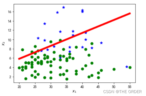
6 绘制决策边界
%matplotlib inline
#绘制决策边界
for i in range(m):
    x=X[i]
    if y[i]==1:
        pl.scatter(x[1],x[2],marker='*',color='blue',s=50)
    else:
        pl.scatter(x[1],x[2],marker='o',color='green',s=50)

hSpots=np.linspace(X[:,1].min(),X[:,1].max(),100)
theta0,theta1,theta2=thetas[-1]

vSpots=-(theta0+theta1*hSpots)/theta2
pl.plot(hSpots,vSpots,color='red',linewidth=5)
pl.xlabel(r'$x_1$')
pl.ylabel(r'$x_2$')
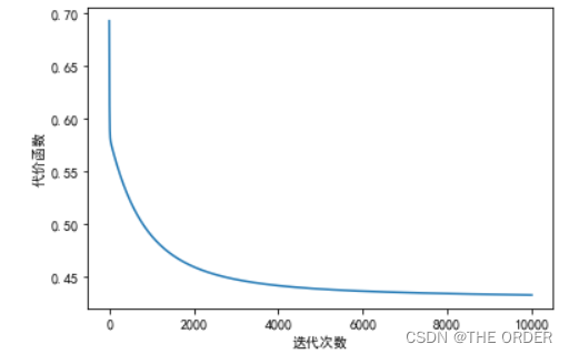
7 绘制误差曲线和参数theta变化
#绘制误差曲线
pl.plot(range(len(errors)),errors)
pl.xlabel(u’迭代次数’)
pl.ylabel(u’代价函数’)
pl.show()
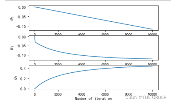
#绘制参数theta变化
thetasFig,ax=pl.subplots(len(thetas[0]))
thetas=np.asarray(thetas)
for idx,sp in enumerate(ax):
    thetaList=thetas[:,idx]
    sp.plot(range(len(thetaList)),thetaList)
    sp.set_xlabel('Number of iteration')
    sp.set_ylabel(r'$\theta_%d$'%idx)

【声明】本内容来自华为云开发者社区博主,不代表华为云及华为云开发者社区的观点和立场。转载时必须标注文章的来源(华为云社区)、文章链接、文章作者等基本信息,否则作者和本社区有权追究责任。如果您发现本社区中有涉嫌抄袭的内容,欢迎发送邮件进行举报,并提供相关证据,一经查实,本社区将立刻删除涉嫌侵权内容,举报邮箱:
cloudbbs@huaweicloud.com
- 点赞
- 收藏
- 关注作者
评论(0)