本节是python实现一元回归的代码部分，理论参考链接: link.
代码下载地址link.
代码可直接赋值运行，如有问题请留言

1 环境准备

import numpy as np
import matplotlib.pyplot as pl
import matplotlib
matplotlib.rcParams['font.sans-serif']='SimHei'
matplotlib.rcParams['font.family']='sans-serif'
matplotlib.rcParams['axes.unicode_minus']=False

这些是需要的python组件和画图需要的包，matplotlib是画图的设置

2 读取文件方法设置

def loadDataset(filename):
    X=[]
    Y=[]
    with open(filename,'rb') as f:
        for idx,line in enumerate(f):
            line=line.decode('utf-8').strip()
            if not line:
                continue
                
            eles=line.split(',')
            
            if idx==0:
                numFea=len(eles)
                
            eles=list(map(float,eles))#map返回一个迭代对象
            
            X.append(eles[:-1])
            Y.append([eles[-1]])
    return np.array(X),np.array(Y)
    ```

# 3 预测值方法
def h(theta,X):
    return np.dot(X,theta)

# 4 完成方法设计

def J(theta,X,Y):
    return np.sum(np.dot((h(theta,X)-Y).T,(h(theta,X)-Y))/(2*m))

# 5 梯度下降方法

def bgd(alpha,maxloop,epsilon,X,Y):
m,n=X.shape

theta=np.zeros((2,1))

count=0
converged=False
error=np.inf
errors=[]
thetas={0:[theta[0,0]],1:[theta[1,0]]}

while count<=maxloop:
    if(converged):
        break
    
    count=count+1
    temp1=theta[0,0]-alpha/m*(h(theta,X)-Y).sum()
    temp2=theta[1,0]-alpha/m*(np.dot(X[:,1][:,np.newaxis].T,(h(theta,X)-Y))).sum()
    
    #同步更新
    theta[0,0]=temp1
    theta[1,0]=temp2
    thetas[0].append(temp1)
    thetas[1].append(temp2)
    
    error=J(theta,X,Y)
    errors.append(error)
    
    if(error<epsilon):
        converged=True
return theta,errors,thetas
```

6 读取文件

先预览下读取的数据，这里用的一组不太好的数据

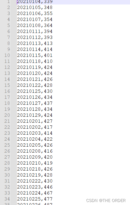
X,Y=loadDataset('./data/price_diff.csv')
print(X.shape)
print(Y.shape)

(243, 1)
(243, 1)

m,n=X.shape
X=np.concatenate((np.ones((m,1)),X),axis=1)
X.shape

(243, 2)

7 模型参数设置

alpha=0.000000000000000003
maxloop=3000
epsilon=0.01
result=bgd(alpha,maxloop,epsilon,X,Y)
theta,errors,thetas=result

xCopy=X.copy()
xCopy.sort(0)
yHat=h(theta,xCopy)
xCopy[:,1].shape,yHat.shape,theta.shape

((243,), (243, 1), (2, 1))

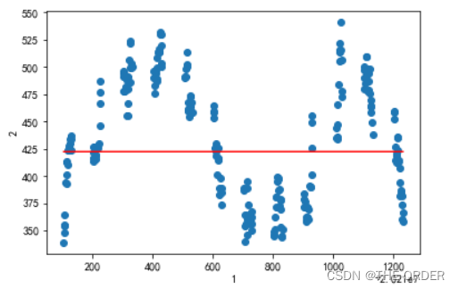
8 结果绘图

pl.xlabel(u'1')
pl.ylabel(u'2')
pl.plot(xCopy[:,1],yHat,color='red')
pl.scatter(X[:,1].flatten(),Y.T.flatten())
pl.show()

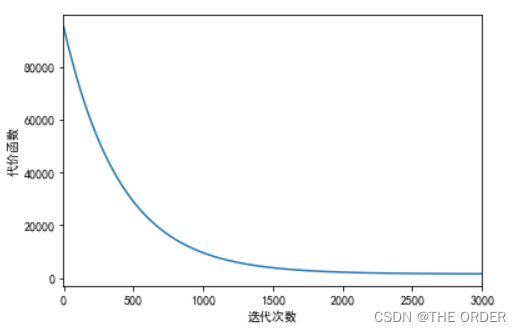
误差与迭代次数绘图

pl.xlim(-1,3000)

pl.xlabel(u'迭代次数')
pl.ylabel(u'代价函数')
pl.plot(range(len(errors)),errors)
pl.show()