- 微信
- 微博
  
  分享文章到微博
- 复制链接
  
  复制链接到剪贴板

【PyTorch基础教程1】线性模型（学不会来打我啊）

野猪佩奇996 发表于 2022/01/23 00:08:53 2022/01/23

【摘要】文章目录一、线性模型二、绘图工具三、作业Reference 一、线性模型不要小看简单线性模型哈哈，虽然这讲我们还没正式用到pytorch，但是用到的前向传播、损失函数、两种绘loss图...

文章目录

一、线性模型
二、绘图工具
三、作业
Reference

一、线性模型

不要小看简单线性模型哈哈，虽然这讲我们还没正式用到pytorch，但是用到的前向传播、损失函数、两种绘loss图等方法在后面是很常用的。
对下面的代码说明：

zip函数可以将x_data和y_data组合元组列表，在for循环中每次遍历就是对于列表中的每个元组。
函数forward()中，有一个变量w。这个变量最终的值是从for循环中传入的。

# -*- coding: utf-8 -*-
"""
Created on Tue Oct 12 14:30:13 2021

@author: 86493
"""
import numpy as np
import matplotlib.pyplot as plt

x_data = [1.0, 2.0, 3.0]
y_data = [2.0, 4.0, 6.0]

def forward(x):
    return x * w

def loss(x, y):
    y_pred = forward(x)
    return (y_pred - y) * (y_pred - y)

# 保存权重
w_list = []
# 保存权重的损失函数值
mse_list = []

# 穷举w值对应的损失函数MSE
for w in np.arange(0.0, 4.1, 0.1):
    print('w = ', w)
    loss_sum = 0
    for x_val, y_val in zip(x_data, y_data):
        # 为了打印y预测值，其实loss里也计算了
        y_pred_val = forward(x_val)
        loss_val = loss(x_val, y_val)
        loss_sum += loss_val
        print('\t', x_val, y_val,
              y_pred_val, loss_val)
    print('MSE = ', loss_sum / 3)
    print('='*60)
    w_list.append(w)
    mse_list.append(loss_sum / 3)
    

 # 绘loss变化图，横坐标是w，纵坐标是loss
plt.plot(w_list, mse_list)
plt.ylabel('Loss')
plt.xlabel('w')
plt.show()

  
 
  1
  2
  3
  4
  5
  6
  7
  8
  9
  10
  11
  12
  13
  14
  15
  16
  17
  18
  19
  20
  21
  22
  23
  24
  25
  26
  27
  28
  29
  30
  31
  32
  33
  34
  35
  36
  37
  38
  39
  40
  41
  42
  43
  44
  45
  46

刚才对应的打印结果为：

w =  0.0
	 1.0 2.0 0.0 4.0
	 2.0 4.0 0.0 16.0
	 3.0 6.0 0.0 36.0
MSE =  18.666666666666668
============================================================
w =  0.1
	 1.0 2.0 0.1 3.61
	 2.0 4.0 0.2 14.44
	 3.0 6.0 0.30000000000000004 32.49
MSE =  16.846666666666668
============================================================
w =  0.2
	 1.0 2.0 0.2 3.24
	 2.0 4.0 0.4 12.96
	 3.0 6.0 0.6000000000000001 29.160000000000004
MSE =  15.120000000000003
============================================================
w =  0.30000000000000004
	 1.0 2.0 0.30000000000000004 2.8899999999999997
	 2.0 4.0 0.6000000000000001 11.559999999999999
	 3.0 6.0 0.9000000000000001 26.009999999999998
MSE =  13.486666666666665
============================================================
w =  0.4
	 1.0 2.0 0.4 2.5600000000000005
	 2.0 4.0 0.8 10.240000000000002
	 3.0 6.0 1.2000000000000002 23.04
MSE =  11.946666666666667
============================================================
w =  0.5
	 1.0 2.0 0.5 2.25
	 2.0 4.0 1.0 9.0
	 3.0 6.0 1.5 20.25
MSE =  10.5
============================================================
w =  0.6000000000000001
	 1.0 2.0 0.6000000000000001 1.9599999999999997
	 2.0 4.0 1.2000000000000002 7.839999999999999
	 3.0 6.0 1.8000000000000003 17.639999999999993
MSE =  9.146666666666663
============================================================
w =  0.7000000000000001
	 1.0 2.0 0.7000000000000001 1.6899999999999995
	 2.0 4.0 1.4000000000000001 6.759999999999998
	 3.0 6.0 2.1 15.209999999999999
MSE =  7.886666666666666
============================================================
w =  0.8
	 1.0 2.0 0.8 1.44
	 2.0 4.0 1.6 5.76
	 3.0 6.0 2.4000000000000004 12.959999999999997
MSE =  6.719999999999999
============================================================
w =  0.9
	 1.0 2.0 0.9 1.2100000000000002
	 2.0 4.0 1.8 4.840000000000001
	 3.0 6.0 2.7 10.889999999999999
MSE =  5.646666666666666
============================================================
w =  1.0
	 1.0 2.0 1.0 1.0
	 2.0 4.0 2.0 4.0
	 3.0 6.0 3.0 9.0
MSE =  4.666666666666667
============================================================
w =  1.1
	 1.0 2.0 1.1 0.8099999999999998
	 2.0 4.0 2.2 3.2399999999999993
	 3.0 6.0 3.3000000000000003 7.289999999999998
MSE =  3.779999999999999
============================================================
w =  1.2000000000000002
	 1.0 2.0 1.2000000000000002 0.6399999999999997
	 2.0 4.0 2.4000000000000004 2.5599999999999987
	 3.0 6.0 3.6000000000000005 5.759999999999997
MSE =  2.986666666666665
============================================================
w =  1.3
	 1.0 2.0 1.3 0.48999999999999994
	 2.0 4.0 2.6 1.9599999999999997
	 3.0 6.0 3.9000000000000004 4.409999999999998
MSE =  2.2866666666666657
============================================================
w =  1.4000000000000001
	 1.0 2.0 1.4000000000000001 0.3599999999999998
	 2.0 4.0 2.8000000000000003 1.4399999999999993
	 3.0 6.0 4.2 3.2399999999999993
MSE =  1.6799999999999995
============================================================
w =  1.5
	 1.0 2.0 1.5 0.25
	 2.0 4.0 3.0 1.0
	 3.0 6.0 4.5 2.25
MSE =  1.1666666666666667
============================================================
w =  1.6
	 1.0 2.0 1.6 0.15999999999999992
	 2.0 4.0 3.2 0.6399999999999997
	 3.0 6.0 4.800000000000001 1.4399999999999984
MSE =  0.746666666666666
============================================================
w =  1.7000000000000002
	 1.0 2.0 1.7000000000000002 0.0899999999999999
	 2.0 4.0 3.4000000000000004 0.3599999999999996
	 3.0 6.0 5.1000000000000005 0.809999999999999
MSE =  0.4199999999999995
============================================================
w =  1.8
	 1.0 2.0 1.8 0.03999999999999998
	 2.0 4.0 3.6 0.15999999999999992
	 3.0 6.0 5.4 0.3599999999999996
MSE =  0.1866666666666665
============================================================
w =  1.9000000000000001
	 1.0 2.0 1.9000000000000001 0.009999999999999974
	 2.0 4.0 3.8000000000000003 0.0399999999999999
	 3.0 6.0 5.7 0.0899999999999999
MSE =  0.046666666666666586
============================================================
w =  2.0
	 1.0 2.0 2.0 0.0
	 2.0 4.0 4.0 0.0
	 3.0 6.0 6.0 0.0
MSE =  0.0
============================================================
w =  2.1
	 1.0 2.0 2.1 0.010000000000000018
	 2.0 4.0 4.2 0.04000000000000007
	 3.0 6.0 6.300000000000001 0.09000000000000043
MSE =  0.046666666666666835
============================================================
w =  2.2
	 1.0 2.0 2.2 0.04000000000000007
	 2.0 4.0 4.4 0.16000000000000028
	 3.0 6.0 6.6000000000000005 0.36000000000000065
MSE =  0.18666666666666698
============================================================
w =  2.3000000000000003
	 1.0 2.0 2.3000000000000003 0.09000000000000016
	 2.0 4.0 4.6000000000000005 0.36000000000000065
	 3.0 6.0 6.9 0.8100000000000006
MSE =  0.42000000000000054
============================================================
w =  2.4000000000000004
	 1.0 2.0 2.4000000000000004 0.16000000000000028
	 2.0 4.0 4.800000000000001 0.6400000000000011
	 3.0 6.0 7.200000000000001 1.4400000000000026
MSE =  0.7466666666666679
============================================================
w =  2.5
	 1.0 2.0 2.5 0.25
	 2.0 4.0 5.0 1.0
	 3.0 6.0 7.5 2.25
MSE =  1.1666666666666667
============================================================
w =  2.6
	 1.0 2.0 2.6 0.3600000000000001
	 2.0 4.0 5.2 1.4400000000000004
	 3.0 6.0 7.800000000000001 3.2400000000000024
MSE =  1.6800000000000008
============================================================
w =  2.7
	 1.0 2.0 2.7 0.49000000000000027
	 2.0 4.0 5.4 1.960000000000001
	 3.0 6.0 8.100000000000001 4.410000000000006
MSE =  2.2866666666666693
============================================================
w =  2.8000000000000003
	 1.0 2.0 2.8000000000000003 0.6400000000000005
	 2.0 4.0 5.6000000000000005 2.560000000000002
	 3.0 6.0 8.4 5.760000000000002
MSE =  2.986666666666668
============================================================
w =  2.9000000000000004
	 1.0 2.0 2.9000000000000004 0.8100000000000006
	 2.0 4.0 5.800000000000001 3.2400000000000024
	 3.0 6.0 8.700000000000001 7.290000000000005
MSE =  3.780000000000003
============================================================
w =  3.0
	 1.0 2.0 3.0 1.0
	 2.0 4.0 6.0 4.0
	 3.0 6.0 9.0 9.0
MSE =  4.666666666666667
============================================================
w =  3.1
	 1.0 2.0 3.1 1.2100000000000002
	 2.0 4.0 6.2 4.840000000000001
	 3.0 6.0 9.3 10.890000000000004
MSE =  5.646666666666668
============================================================
w =  3.2
	 1.0 2.0 3.2 1.4400000000000004
	 2.0 4.0 6.4 5.760000000000002
	 3.0 6.0 9.600000000000001 12.96000000000001
MSE =  6.720000000000003
============================================================
w =  3.3000000000000003
	 1.0 2.0 3.3000000000000003 1.6900000000000006
	 2.0 4.0 6.6000000000000005 6.7600000000000025
	 3.0 6.0 9.9 15.210000000000003
MSE =  7.886666666666668
============================================================
w =  3.4000000000000004
	 1.0 2.0 3.4000000000000004 1.960000000000001
	 2.0 4.0 6.800000000000001 7.840000000000004
	 3.0 6.0 10.200000000000001 17.640000000000008
MSE =  9.14666666666667
============================================================
w =  3.5
	 1.0 2.0 3.5 2.25
	 2.0 4.0 7.0 9.0
	 3.0 6.0 10.5 20.25
MSE =  10.5
============================================================
w =  3.6
	 1.0 2.0 3.6 2.5600000000000005
	 2.0 4.0 7.2 10.240000000000002
	 3.0 6.0 10.8 23.040000000000006
MSE =  11.94666666666667
============================================================
w =  3.7
	 1.0 2.0 3.7 2.8900000000000006
	 2.0 4.0 7.4 11.560000000000002
	 3.0 6.0 11.100000000000001 26.010000000000016
MSE =  13.486666666666673
============================================================
w =  3.8000000000000003
	 1.0 2.0 3.8000000000000003 3.240000000000001
	 2.0 4.0 7.6000000000000005 12.960000000000004
	 3.0 6.0 11.4 29.160000000000004
MSE =  15.120000000000005
============================================================
w =  3.9000000000000004
	 1.0 2.0 3.9000000000000004 3.610000000000001
	 2.0 4.0 7.800000000000001 14.440000000000005
	 3.0 6.0 11.700000000000001 32.49000000000001
MSE =  16.84666666666667
============================================================
w =  4.0
	 1.0 2.0 4.0 4.0
	 2.0 4.0 8.0 16.0
	 3.0 6.0 12.0 36.0
MSE =  18.666666666666668
============================================================

  
 
  1
  2
  3
  4
  5
  6
  7
  8
  9
  10
  11
  12
  13
  14
  15
  16
  17
  18
  19
  20
  21
  22
  23
  24
  25
  26
  27
  28
  29
  30
  31
  32
  33
  34
  35
  36
  37
  38
  39
  40
  41
  42
  43
  44
  45
  46
  47
  48
  49
  50
  51
  52
  53
  54
  55
  56
  57
  58
  59
  60
  61
  62
  63
  64
  65
  66
  67
  68
  69
  70
  71
  72
  73
  74
  75
  76
  77
  78
  79
  80
  81
  82
  83
  84
  85
  86
  87
  88
  89
  90
  91
  92
  93
  94
  95
  96
  97
  98
  99
  100
  101
  102
  103
  104
  105
  106
  107
  108
  109
  110
  111
  112
  113
  114
  115
  116
  117
  118
  119
  120
  121
  122
  123
  124
  125
  126
  127
  128
  129
  130
  131
  132
  133
  134
  135
  136
  137
  138
  139
  140
  141
  142
  143
  144
  145
  146
  147
  148
  149
  150
  151
  152
  153
  154
  155
  156
  157
  158
  159
  160
  161
  162
  163
  164
  165
  166
  167
  168
  169
  170
  171
  172
  173
  174
  175
  176
  177
  178
  179
  180
  181
  182
  183
  184
  185
  186
  187
  188
  189
  190
  191
  192
  193
  194
  195
  196
  197
  198
  199
  200
  201
  202
  203
  204
  205
  206
  207
  208
  209
  210
  211
  212
  213
  214
  215
  216
  217
  218
  219
  220
  221
  222
  223
  224
  225
  226
  227
  228
  229
  230
  231
  232
  233
  234
  235
  236
  237
  238
  239
  240
  241
  242
  243
  244
  245
  246

二、绘图工具

在深度学习中，我们一般没有打印上面这种loss图（一般横坐标为epoch，而上面这种图可以用于检测最优超参数是多少），下图这里loss虽然随着epoch增大而减少，但是在开发集上的效果却可能是先减小后增大的，所以应该找中间这个画竖线的点。

PS：可以学习模型训练可视化visdom工具，训练还要注意存盘的问题（如防止要训练7天，但在第6天报错了）。

画图除了用matplotlib.pyplot，还经常使用pandas的dataframe.plot，如下：

# 增加loss折线图
import pandas as pd
df = pd.DataFrame(columns = ["Loss"]) # columns列名
df.index.name = "Epoch" 
for epoch in range(1, 201):
    loss = train()
    #df.loc[epoch] = loss.item()
    df.loc[epoch] = loss.item()
df.plot() 

  
 
  1
  2
  3
  4
  5
  6
  7
  8
  9

上面这种loss图也是最典型的.

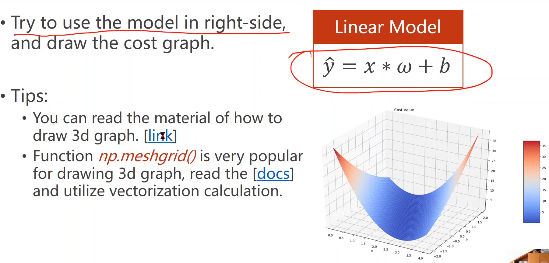
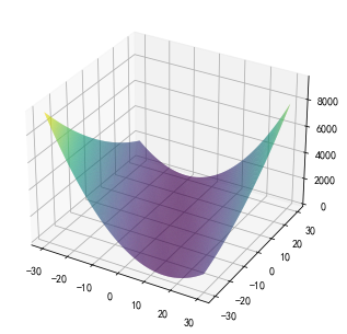
三、作业

实现线性模型（ $y = w x + b$ ）并输出loss的3D图像。

# -*- coding: utf-8 -*-
"""
Created on Tue Oct 12 17:04:46 2021

@author: 86493
"""
import numpy as np
import matplotlib.pyplot as plt;
from mpl_toolkits.mplot3d import Axes3D
from matplotlib import cm

x_data = [1.0, 2.0, 3.0]
y_data = [2.0, 4.0, 6.0]

# 线性模型,多了个b
def forward(x,w,b):
    return x * w + b

# 损失函数，此处没变
def loss(x, y, w, b):
    y_pred = forward(x, w, b)
    return (y_pred - y) * (y_pred - y)

# 单独写出mse函数，为了计算不同w和b情况下对应的mse
def mse(w,b):
    l_sum = 0
    for x_val, y_val in zip(x_data, y_data):
        y_pred_val = forward(x_val,w,b)
        loss_val = loss(x_val, y_val,w,b)
        l_sum += loss_val
        print('\t', x_val, y_val, y_pred_val, loss_val)
    print('MSE=', l_sum / 3)
    return  l_sum/3

#迭代取值，计算每个w取值下的x，y，y_pred,loss_val
mse_list = []


# 画图

# 1.定义网格化数据
b_list=np.arange(-30,30,0.1)
w_list=np.arange(-30,30,0.1);

# 2.生成网格化数据
xx, yy = np.meshgrid(b_list, w_list, sparse=False, indexing='xy')

# 3.每个点的对应高度
zz=mse(xx,yy)

fig = plt.figure()
ax = Axes3D(fig)
ax.plot_surface(xx, yy, zz, 
                rstride=1,   # rows stride 指定行的跨度为1，只能是int
                cstride=1,   # columns stride 指定列的跨度为1
                cmap=cm.viridis) # 设置曲面的颜色
plt.show()

  
 
  1
  2
  3
  4
  5
  6
  7
  8
  9
  10
  11
  12
  13
  14
  15
  16
  17
  18
  19
  20
  21
  22
  23
  24
  25
  26
  27
  28
  29
  30
  31
  32
  33
  34
  35
  36
  37
  38
  39
  40
  41
  42
  43
  44
  45
  46
  47
  48
  49
  50
  51
  52
  53
  54
  55
  56
  57

Reference

[1] 3D图绘制：https://matplotlib.org/stable/tutorials/toolkits/mplot3d.html
[2] https://numpy.org/doc/stable/reference/generated/numpy.meshgrid.html#numpy.meshgrid
[3] Matplotlib3D作图-plot_surface(), .contourf(), plt.colorbar()
[4]【matplotlib】如何进行颜色设置选择cmap
[5] https://blog.csdn.net/Pin_BOY/article/details/119707358
[6] http://biranda.top/archives/page/2/

文章来源: andyguo.blog.csdn.net，作者：山顶夕景，版权归原作者所有，如需转载，请联系作者。

原文链接：andyguo.blog.csdn.net/article/details/120724013

点赞
收藏
关注作者

0/1000

抱歉，系统识别当前为高风险访问，暂不支持该操作

全部回复

上滑加载中

设置昵称

在此一键设置昵称，即可参与社区互动！

*长度不超过10个汉字或20个英文字符，设置后3个月内不可修改。

确认取消

加入云驻计划，成为创作者

华为云周边好礼
免费体验产品
特殊身份标识
线下官方门票
内部专家零距离
与10000+优质创作者共同成长

立即加入