Matplotlib绘制简单函数的梯度下降法

➤01 一维函数
使用matplotlib的绘制函数是非常方便和容易的。
下面这个有趣的例子来自于飞浆PaddlePaddle深度学习实战P20中的例子。
1.简单的例子
演示了对于 y = x 2 y = x^2 y=x2函数通过局部的梯度下降方法来逐步获得全局极小值。
#!/usr/local/bin/python
# -*- coding: gbk -*-
#============================================================
# DEMO1.PY                     -- by Dr. ZhuoQing 2020-11-16
#
# Note:
#============================================================

from headm import *

#------------------------------------------------------------
def func(x):
    return square(x)

def dfunc(x):
    return 2 * x                    # Derivative of x**2

#------------------------------------------------------------
def gradient_descent(x_start, func_deri, epochs, learning_rate):
    theta_x = zeros(epochs+1)
    temp_x = x_start
    theta_x[0] = temp_x

    for i in range(epochs):
        deri_x = func_deri(temp_x)
        delta = -deri_x * learning_rate
        temp_x = temp_x + delta
        theta_x[i+1] = temp_x

    return theta_x

#------------------------------------------------------------
def mat_plot():
    line_x = linspace(-5, 5, 100)
    line_y = func(line_x)

    x_start = -5
    epochs = 5
    lr = 0.3
    x = gradient_descent(x_start, dfunc, epochs, lr)

    color = 'r'
    plt.plot(line_x, line_y, c='b')
    plt.plot(x, func(x), c=color, linestyle='--', linewidth=1, label='lr={}'.format(lr))
    plt.scatter(x, func(x), color=color)
    plt.xlabel('x')
    plt.ylabel('x^2')
    plt.legend()
    plt.show()

mat_plot()

#------------------------------------------------------------
#        END OF FILE : DEMO1.PY
#============================================================
- 1
- 2
- 3
- 4
- 5
- 6
- 7
- 8
- 9
- 10
- 11
- 12
- 13
- 14
- 15
- 16
- 17
- 18
- 19
- 20
- 21
- 22
- 23
- 24
- 25
- 26
- 27
- 28
- 29
- 30
- 31
- 32
- 33
- 34
- 35
- 36
- 37
- 38
- 39
- 40
- 41
- 42
- 43
- 44
- 45
- 46
- 47
- 48
- 49
- 50
- 51
- 52
- 53
- 54
- 55

▲ 绘制x**2梯度下降
2.绘制不同Learning Rate的梯度下降过程
绘制不同Learning Rate下的梯度下降方法对应的迭代过程。

▲ 学习速率从0.01增加到1.5
def mat_plot(learning_rate=0.3):
    line_x = linspace(-5, 5, 100)
    line_y = func(line_x)

    x_start = -5
    epochs = 10
    lr = learning_rate
    x = gradient_descent(x_start, dfunc, epochs, lr)

    color = 'r'
    plt.clf()
    plt.plot(line_x, line_y, c='b')
    plt.plot(x, func(x), c=color, linestyle='--', linewidth=1, label='lr=%4.2f'%lr)
    plt.scatter(x, func(x), color=color)
    plt.xlabel('x')
    plt.ylabel('x^2')
    plt.legend(loc='upper right')
#    plt.show()
    plt.draw()
    plt.pause(.001)

#------------------------------------------------------------
pltgif = PlotGIF()

for lr in linspace(0.01, 1.5, 100):
    mat_plot(lr)

    if lr > 0.01:
        pltgif.append(plt)

pltgif.save(r'd:\temp\1.gif')
- 1
- 2
- 3
- 4
- 5
- 6
- 7
- 8
- 9
- 10
- 11
- 12
- 13
- 14
- 15
- 16
- 17
- 18
- 19
- 20
- 21
- 22
- 23
- 24
- 25
- 26
- 27
- 28
- 29
- 30
- 31
- 32
- 33
➤02 二维函数
根据 Python 中的3Dplot 中给出的轮廓函数,来进行梯度下降的实验。
1.函数
Z ( x , y ) = e − ( x + 1 ) 2 − ( y + 0.5 ) 2 − e − ( x − 1 ) 2 − ( y − 0.5 ) 2 Z\left( {x,y} \right) = e^{ - \left( {x + 1} \right)^2 - \left( {y + 0.5} \right)^2 } - e^{ - \left( {x - 1} \right)^2 - \left( {y - 0.5} \right)^2 } Z(x,y)=e−(x+1)2−(y+0.5)2−e−(x−1)2−(y−0.5)2
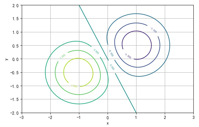
▲ 二维函数的等高线图
def func(x,y):
    res = exp(-(x+1)**2-(y+0.5)**2)-exp(-(x-1)**2-(y-0.5)**2)
    return res*2

def dfunc(x,y):
    dx = -2*(x+1)*exp(-(x+1)**2-(y+0.5)**2) + 2*(x-1)*exp(-(x-1)**2-(y-0.5)**2)
    dy = -2*(y+0.5)*exp(-(x+1)**2-(y+0.5)**2) + 2*(y-0.5)*exp(-(x-1)**2-(y-0.5)**2)
    return dx*2,dy*2

def gradient_descent(x_start, y_start, epochs, learning_rate):
    theta_x = []
    theta_y = []
    temp_x = x_start
    temp_y = y_start

    theta_x.append(temp_x)
    theta_y.append(temp_y)

    for i in range(epochs):
        dx,dy = dfunc(temp_x, temp_y)
        temp_x = temp_x - dx*learning_rate
        temp_y = temp_y - dy*learning_rate

        theta_x.append(temp_x)
        theta_y.append(temp_y)

    return theta_x, theta_y

#------------------------------------------------------------
def mat_plot(learning_rate=0.3):
    delta = 0.025
    x = arange(-3.0, 3.0, delta)
    y = arange(-3.0, 3.0, delta)
    X,Y = meshgrid(x,y)
    Z = func(X, Y)

    CS = plt.contour(X, Y, Z)
    plt.clabel(CS, inline=0.5, fontsize=6)
    plt.xlabel('x')
    plt.ylabel('y')
    plt.grid(True)
    plt.axis([-3, 3, -2, 2])
    plt.tight_layout()
    plt.show()
- 1
- 2
- 3
- 4
- 5
- 6
- 7
- 8
- 9
- 10
- 11
- 12
- 13
- 14
- 15
- 16
- 17
- 18
- 19
- 20
- 21
- 22
- 23
- 24
- 25
- 26
- 27
- 28
- 29
- 30
- 31
- 32
- 33
- 34
- 35
- 36
- 37
- 38
- 39
- 40
- 41
- 42
- 43
- 44
- 45

函数Z(x,y)对x,y求偏导数:
∂ Z ∂ x = ( − 2 x − 2 ) e − ( x + 1 ) 2 − ( y + 0.5 ) 2 − ( − 2 x + 2 ) e − ( x − 1 ) 2 − ( y − 0.5 ) 2 {{\partial Z} \over {\partial x}} = \left( { - 2x - 2} \right)e^{ - \left( {x + 1} \right)^2 - \left( {y + 0.5} \right)^2 } - \left( { - 2x + 2} \right)e^{ - \left( {x - 1} \right)^2 - \left( {y - 0.5} \right)^2 } ∂x∂Z=(−2x−2)e−(x+1)2−(y+0.5)2−(−2x+2)e−(x−1)2−(y−0.5)2
∂ Z ∂ y = ( − 2 y − 1.0 ) e − ( x + 1 ) 2 − ( y + 0.5 ) 2 − ( − 2 y + 1.0 ) e − ( x − 1 ) 2 − ( y − 0.5 ) 2 {{\partial Z} \over {\partial y}} = \left( { - 2y - 1.0} \right)e^{ - \left( {x + 1} \right)^2 - \left( {y + 0.5} \right)^2 } - \left( { - 2y + 1.0} \right)e^{ - \left( {x - 1} \right)^2 - \left( {y - 0.5} \right)^2 } ∂y∂Z=(−2y−1.0)e−(x+1)2−(y+0.5)2−(−2y+1.0)e−(x−1)2−(y−0.5)2
from sympy                  import symbols,simplify,expand,print_latex
from sympy                  import diff,exp

#------------------------------------------------------------
x,y,f = symbols('x,y,f')

f=exp(-(x+1)**2-(y+0.5)**2)-exp(-(x-1)**2-(y-0.5)**2)

dfdx = diff(f,x)
dfdy = diff(f,y)

result = dfdy

#------------------------------------------------------------
print_latex(result)
tspexecutepythoncmd("msg2latex")
clipboard.copy(str(result))
- 1
- 2
- 3
- 4
- 5
- 6
- 7
- 8
- 9
- 10
- 11
- 12
- 13
- 14
- 15
- 16
- 17
2.二维梯度下降
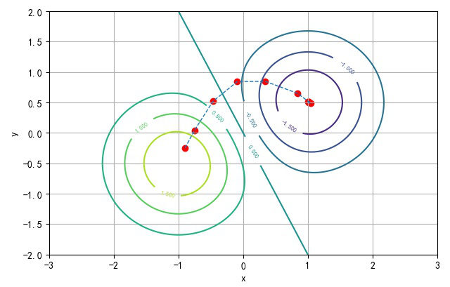
▲ 梯度下降的迭代路线
如下是在Learning-Rate=0.1, Epochs在1 ~ 21的变化的动图。

如下是:Epochs=20,Learning-Rate从0.01到1.2之间变化。

#!/usr/local/bin/python
# -*- coding: gbk -*-
#============================================================
# TEST3.PY                     -- by Dr. ZhuoQing 2020-11-16
#
# Note:
#============================================================

from headm import *

def func(x,y):
    res = exp(-(x+1)**2-(y+0.5)**2)-exp(-(x-1)**2-(y-0.5)**2)
    return res*2

def dfunc(x,y):
    dx = -2*(x+1)*exp(-(x+1)**2-(y+0.5)**2) + 2*(x-1)*exp(-(x-1)**2-(y-0.5)**2)
    dy = -2*(y+0.5)*exp(-(x+1)**2-(y+0.5)**2) + 2*(y-0.5)*exp(-(x-1)**2-(y-0.5)**2)
    return dx*2,dy*2

def gradient_descent(x_start, y_start, epochs, learning_rate):
    theta_x = []
    theta_y = []
    temp_x = x_start
    temp_y = y_start

    theta_x.append(temp_x)
    theta_y.append(temp_y)

    for i in range(epochs):
        dx,dy = dfunc(temp_x, temp_y)
        temp_x = temp_x - dx*learning_rate
        temp_y = temp_y - dy*learning_rate

        theta_x.append(temp_x)
        theta_y.append(temp_y)

    return theta_x, theta_y

#------------------------------------------------------------
def mat_plot(epochs=10, learning_rate=0.3):
    lr = learning_rate
    delta = 0.025
    x = arange(-3.0, 3.0, delta)
    y = arange(-3.0, 3.0, delta)
    X,Y = meshgrid(x,y)
    Z = func(X, Y)

    dx,dy = gradient_descent(-0.9, -0.25, epochs, lr)

    plt.clf()
    plt.scatter(dx, dy, color='r')
    plt.plot(dx, dy, linewidth=1, linestyle='--', label='lr=%4.2f'%lr)

    CS = plt.contour(X, Y, Z)
    plt.clabel(CS, inline=0.5, fontsize=6)
    plt.xlabel('x')
    plt.ylabel('y')
    plt.grid(True)
    plt.axis([-3, 3, -2, 2])
    plt.tight_layout()
    plt.legend(loc='upper right')
    plt.draw()
    plt.pause(.001)

#------------------------------------------------------------

pltgif = PlotGIF()

for i in linspace(0.01, 1.2, 50):
    mat_plot(10, i)
    if i > 0.01:
        pltgif.append(plt)

pltgif.save(r'd:\temp\1.gif')

#------------------------------------------------------------
#        END OF FILE : TEST3.PY
#============================================================
- 1
- 2
- 3
- 4
- 5
- 6
- 7
- 8
- 9
- 10
- 11
- 12
- 13
- 14
- 15
- 16
- 17
- 18
- 19
- 20
- 21
- 22
- 23
- 24
- 25
- 26
- 27
- 28
- 29
- 30
- 31
- 32
- 33
- 34
- 35
- 36
- 37
- 38
- 39
- 40
- 41
- 42
- 43
- 44
- 45
- 46
- 47
- 48
- 49
- 50
- 51
- 52
- 53
- 54
- 55
- 56
- 57
- 58
- 59
- 60
- 61
- 62
- 63
- 64
- 65
- 66
- 67
- 68
- 69
- 70
- 71
- 72
- 73
- 74
- 75
- 76
- 77
- 78

#------------------------------------------------------------
def mat_plot(epochs=10, learning_rate=0.3):
    lr = learning_rate
    delta = 0.025
    x = arange(-3.0, 3.0, delta)
    y = arange(-3.0, 3.0, delta)
    X,Y = meshgrid(x,y)
    Z = func(X, Y)

    dx,dy = gradient_descent(-0.9, -0.25, epochs, lr)

    plt.clf()
    ax = plt.axes(projection='3d')
#    ax.plot_surface(X,Y,Z, cmap='coolwarm')
    ax.contour(X,Y,Z)

    ax.scatter(dx, dy, func(array(dx),array(dy)), color='r')
    ax.plot(dx, dy, func(array(dx), array(dy)), linewidth=1, linestyle='--', label='lr=%4.2f'%lr)

#    CS = plt.contour(X, Y, Z)
#    plt.clabel(CS, inline=0.5, fontsize=6)

    plt.xlabel('x')
    plt.ylabel('y')
    plt.grid(True)
    plt.axis([-3, 3, -2, 2])
    plt.tight_layout()
    plt.legend(loc='upper right')
    plt.draw()
    plt.pause(.1)

#------------------------------------------------------------

pltgif = PlotGIF()

for i in linspace(0.01, 1.2, 100):
    mat_plot(20, i)
    if i > 0.01:
        pltgif.append(plt)

pltgif.save(r'd:\temp\1.gif')

#------------------------------------------------------------
#        END OF FILE : TEST3.PY
#============================================================
- 1
- 2
- 3
- 4
- 5
- 6
- 7
- 8
- 9
- 10
- 11
- 12
- 13
- 14
- 15
- 16
- 17
- 18
- 19
- 20
- 21
- 22
- 23
- 24
- 25
- 26
- 27
- 28
- 29
- 30
- 31
- 32
- 33
- 34
- 35
- 36
- 37
- 38
- 39
- 40
- 41
- 42
- 43
- 44
- 45
- 46
文章来源: zhuoqing.blog.csdn.net,作者:卓晴,版权归原作者所有,如需转载,请联系作者。
原文链接:zhuoqing.blog.csdn.net/article/details/109732365

- 点赞
- 收藏
- 关注作者
评论(0)