回归:预测燃油效率


回归:预测燃油效率
在一个回归问题中,我们的目标是预测一个连续值的输出,比如价格或概率。这与一个分类问题形成对比,我们的目标是从一系列类中选择一个类(例如,一张图片包含一个苹果或一个橘子,识别图片中的水果)。
本笔记本使用经典的[auto-mpg](https://archive.ics.uci.edu/ml/datasets/auto+mpg)数据集,建立了预测70年代末和80年代初汽车燃油效率的模型。为了做到这一点,我们将为该模型提供从那个时期开始的许多汽车的描述。此描述包括以下属性:气缸、排量、马力和重量。
此示例使用“tf.keras”API,有关详细信息,请参阅[本指南](https://www.tensorflow.org/guide/keras)。
import pathlib
import matplotlib.pyplot as plt
import pandas as pd
import seaborn as sns
import keras
from keras import layers
%matplotlib inline
- 1
- 2
- 3
- 4
- 5
- 6
- 7
- 8
The Auto MPG dataset
The dataset is available from the UCI Machine Learning Repository.
Get the data
First download the dataset.
dataset_path = keras.utils.get_file("auto-mpg.data", "https://archive.ics.uci.edu/ml/machine-learning-databases/auto-mpg/auto-mpg.data")
dataset_path
- 1
- 2
'C:\\Users\\YIUYE\\.keras\\datasets\\auto-mpg.data'
- 1
Import it using pandas
column_names = ['MPG','Cylinders','Displacement','Horsepower','Weight', 'Acceleration', 'Model Year', 'Origin']
raw_dataset = pd.read_csv(dataset_path, names=column_names, na_values = "?", comment='\t', sep=" ", skipinitialspace=True)

dataset = raw_dataset.copy()
dataset.tail()
- 1
- 2
- 3
- 4
- 5
- 6
- 7
- 8
| MPG | Cylinders | Displacement | Horsepower | Weight | Acceleration | Model Year | Origin | |
|---|---|---|---|---|---|---|---|---|
| 393 | 27.0 | 4 | 140.0 | 86.0 | 2790.0 | 15.6 | 82 | 1 |
| 394 | 44.0 | 4 | 97.0 | 52.0 | 2130.0 | 24.6 | 82 | 2 |
| 395 | 32.0 | 4 | 135.0 | 84.0 | 2295.0 | 11.6 | 82 | 1 |
| 396 | 28.0 | 4 | 120.0 | 79.0 | 2625.0 | 18.6 | 82 | 1 |
| 397 | 31.0 | 4 | 119.0 | 82.0 | 2720.0 | 19.4 | 82 | 1 |
Clean the data
The dataset contains a few unknown values.
dataset.isnull().sum()
- 1
MPG 0
Cylinders 0
Displacement 0
Horsepower 6
Weight 0
Acceleration 0
Model Year 0
Origin 0
dtype: int64
- 1
- 2
- 3
- 4
- 5
- 6
- 7
- 8
- 9
To keep this initial tutorial simple drop those rows.
dataset = dataset.dropna()
- 1
- 2
The "Origin" column is really categorical, not numeric. So convert that to a one-hot:
origin = dataset.pop('Origin')
- 1
dataset['USA'] = (origin == 1)*1.0
dataset['Europe'] = (origin == 2)*1.0
dataset['Japan'] = (origin == 3)*1.0
dataset.tail()
- 1
- 2
- 3
- 4
| MPG | Cylinders | Displacement | Horsepower | Weight | Acceleration | Model Year | USA | Europe | Japan | |
|---|---|---|---|---|---|---|---|---|---|---|
| 393 | 27.0 | 4 | 140.0 | 86.0 | 2790.0 | 15.6 | 82 | 1.0 | 0.0 | 0.0 |
| 394 | 44.0 | 4 | 97.0 | 52.0 | 2130.0 | 24.6 | 82 | 0.0 | 1.0 | 0.0 |
| 395 | 32.0 | 4 | 135.0 | 84.0 | 2295.0 | 11.6 | 82 | 1.0 | 0.0 | 0.0 |
| 396 | 28.0 | 4 | 120.0 | 79.0 | 2625.0 | 18.6 | 82 | 1.0 | 0.0 | 0.0 |
| 397 | 31.0 | 4 | 119.0 | 82.0 | 2720.0 | 19.4 | 82 | 1.0 | 0.0 | 0.0 |
现在将数据集拆分为一个训练集和一个测试集。
我们将在模型的最终评估中使用测试集。
train_dataset = dataset.sample(frac=0.8,random_state=0)
test_dataset = dataset.drop(train_dataset.index)
- 1
- 2
sns.pairplot(train_dataset[[ "Cylinders", "Displacement", "Weight"]], diag_kind="kde")
sns.set()
- 1
- 2

Also look at the overall statistics:
train_stats = train_dataset.describe()
train_stats.pop("MPG")
train_stats = train_stats.transpose()
train_stats
- 1
- 2
- 3
- 4
| count | mean | std | min | 25% | 50% | 75% | max | |
|---|---|---|---|---|---|---|---|---|
| Cylinders | 314.0 | 5.477707 | 1.699788 | 3.0 | 4.00 | 4.0 | 8.00 | 8.0 |
| Displacement | 314.0 | 195.318471 | 104.331589 | 68.0 | 105.50 | 151.0 | 265.75 | 455.0 |
| Horsepower | 314.0 | 104.869427 | 38.096214 | 46.0 | 76.25 | 94.5 | 128.00 | 225.0 |
| Weight | 314.0 | 2990.251592 | 843.898596 | 1649.0 | 2256.50 | 2822.5 | 3608.00 | 5140.0 |
| Acceleration | 314.0 | 15.559236 | 2.789230 | 8.0 | 13.80 | 15.5 | 17.20 | 24.8 |
| Model Year | 314.0 | 75.898089 | 3.675642 | 70.0 | 73.00 | 76.0 | 79.00 | 82.0 |
| USA | 314.0 | 0.624204 | 0.485101 | 0.0 | 0.00 | 1.0 | 1.00 | 1.0 |
| Europe | 314.0 | 0.178344 | 0.383413 | 0.0 | 0.00 | 0.0 | 0.00 | 1.0 |
| Japan | 314.0 | 0.197452 | 0.398712 | 0.0 | 0.00 | 0.0 | 0.00 | 1.0 |
Split features from labels
Separate the target value, or “label”, from the features. This label is the value that you will train the model to predict.
train_labels = train_dataset.pop('MPG')
test_labels = test_dataset.pop('MPG')
- 1
- 2
Normalize the data
Look again at the train_stats block above and note how different the ranges of each feature are.
规范化使用不同尺度和范围的特征是一个很好的实践。虽然模型可能在没有特征规范化的情况下收敛,但它使训练变得更加困难,并且使生成的模型依赖于输入中使用的单元的选择。
注意:尽管我们有意只从训练数据集生成这些统计信息,但这些统计信息也将用于规范化测试数据集。我们需要这样做,以将测试数据集投影到模型所训练的相同分发中。
def norm(x):
  return (x - train_stats['mean']) / train_stats['std']
normed_train_data = norm(train_dataset)
normed_test_data = norm(test_dataset)
- 1
- 2
- 3
- 4
def build_model():
  model = keras.Sequential([ layers.Dense(64, activation=tf.nn.relu, input_shape=[len(train_dataset.keys())]), layers.Dense(64, activation=tf.nn.relu), layers.Dense(1)
  ]) optimizer = keras.optimizers.RMSprop(0.001) model.compile(loss='mean_squared_error', optimizer=optimizer, metrics=['mean_absolute_error', 'mean_squared_error'])
  return model
- 1
- 2
- 3
- 4
- 5
- 6
- 7
- 8
- 9
- 10
- 11
- 12
- 13
model = build_model()
- 1
model.summary()
- 1
_________________________________________________________________
Layer (type) Output Shape Param # =================================================================
dense_10 (Dense) (None, 64) 640 _________________________________________________________________
dense_11 (Dense) (None, 64) 4160 _________________________________________________________________
dense_12 (Dense) (None, 1) 65 =================================================================
Total params: 4,865
Trainable params: 4,865
Non-trainable params: 0
_________________________________________________________________
- 1
- 2
- 3
- 4
- 5
- 6
- 7
- 8
- 9
- 10
- 11
- 12
- 13
Now try out the model. Take a batch of 10 examples from the training data and call model.predict on it.
example_batch = normed_train_data[:10]
example_result = model.predict(example_batch)
example_result
- 1
- 2
- 3
array([[-0.03468257], [-0.01342154], [-0.15384783], [-0.18010283], [ 0.03922582], [-0.12172151], [ 0.10603201], [ 0.2442987 ], [ 0.00099315], [ 0.18530795]], dtype=float32)
- 1
- 2
- 3
- 4
- 5
- 6
- 7
- 8
- 9
- 10
It seems to be working, and it produces a result of the expected shape and type.
Train the model
Train the model for 1000 epochs, and record the training and validation accuracy in the history object.
# Display training progress by printing a single dot for each completed epoch
class PrintDot(keras.callbacks.Callback):
  def on_epoch_end(self, epoch, logs): if epoch % 100 == 0: print('') print('.', end='')

EPOCHS = 1000

history = model.fit(
  normed_train_data, train_labels,
  epochs=EPOCHS, validation_split = 0.2, verbose=0,
  callbacks=[PrintDot()])
- 1
- 2
- 3
- 4
- 5
- 6
- 7
- 8
- 9
- 10
- 11
- 12
....................................................................................................
....................................................................................................
....................................................................................................
....................................................................................................
....................................................................................................
....................................................................................................
....................................................................................................
....................................................................................................
....................................................................................................
....................................................................................................
- 1
- 2
- 3
- 4
- 5
- 6
- 7
- 8
- 9
- 10
hist = pd.DataFrame(history.history)
hist['epoch'] = history.epoch
hist.tail()
- 1
- 2
- 3
| loss | mean_absolute_error | mean_squared_error | val_loss | val_mean_absolute_error | val_mean_squared_error | epoch | |
|---|---|---|---|---|---|---|---|
| 995 | 2.075518 | 0.940943 | 2.075518 | 8.913726 | 2.351839 | 8.913726 | 995 |
| 996 | 2.130111 | 0.953561 | 2.130111 | 9.769884 | 2.438282 | 9.769884 | 996 |
| 997 | 2.221040 | 0.951258 | 2.221040 | 9.664708 | 2.382888 | 9.664708 | 997 |
| 998 | 2.301870 | 0.980407 | 2.301870 | 9.934311 | 2.425505 | 9.934311 | 998 |
| 999 | 2.002580 | 0.887644 | 2.002580 | 9.484982 | 2.414742 | 9.484982 | 999 |
def plot_history(history):
  hist = pd.DataFrame(history.history)
  hist['epoch'] = history.epoch plt.figure()
  plt.xlabel('Epoch')
  plt.ylabel('Mean Abs Error [MPG]')
  plt.plot(hist['epoch'], hist['mean_absolute_error'], label='Train Error')
  plt.plot(hist['epoch'], hist['val_mean_absolute_error'], label = 'Val Error')
  plt.ylim([0,5])
  plt.legend() plt.figure()
  plt.xlabel('Epoch')
  plt.ylabel('Mean Square Error [$MPG^2$]')
  plt.plot(hist['epoch'], hist['mean_squared_error'], label='Train Error')
  plt.plot(hist['epoch'], hist['val_mean_squared_error'], label = 'Val Error')
  plt.ylim([0,20])
  plt.legend()
  plt.show()


plot_history(history)
- 1
- 2
- 3
- 4
- 5
- 6
- 7
- 8
- 9
- 10
- 11
- 12
- 13
- 14
- 15
- 16
- 17
- 18
- 19
- 20
- 21
- 22
- 23
- 24
- 25
- 26
- 27


此图显示在大约100个周期后,验证错误几乎没有改善,甚至恶化。让我们更新“model.fit”调用,以便在验证分数没有提高时自动停止培训。我们将使用一个早期的回调来测试每个时代的训练条件。如果一个设定的时间段没有显示出改善,那么自动停止训练。
model = build_model()

# The patience parameter is the amount of epochs to check for improvement
early_stop = keras.callbacks.EarlyStopping(monitor='val_loss', patience=10)

history = model.fit(normed_train_data, train_labels, epochs=EPOCHS, validation_split = 0.2, verbose=0, callbacks=[early_stop, PrintDot()])

plot_history(history)
- 1
- 2
- 3
- 4
- 5
- 6
- 7
- 8
- 9
.................................................
- 1


loss, mae, mse = model.evaluate(normed_test_data, test_labels, verbose=0)

print("Testing set Mean Abs Error: {:5.2f} MPG".format(mae))
- 1
- 2
- 3
Testing set Mean Abs Error: 1.79 MPG
- 1
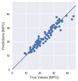
Make predictions
Finally, predict MPG values using data in the testing set:
test_predictions = model.predict(normed_test_data).flatten()

plt.scatter(test_labels, test_predictions)
plt.xlabel('True Values [MPG]')
plt.ylabel('Predictions [MPG]')
plt.axis('equal')
plt.axis('square')
plt.xlim([0,plt.xlim()[1]])
plt.ylim([0,plt.ylim()[1]])
_ = plt.plot([-100, 100], [-100, 100])
- 1
- 2
- 3
- 4
- 5
- 6
- 7
- 8
- 9
- 10
- 11
error = test_predictions - test_labels
plt.hist(error, bins = 25)
plt.xlabel("Prediction Error [MPG]")
_ = plt.ylabel("Count")
- 1
- 2
- 3
- 4

它不是很高斯的,但是我们可以预期,因为样本的数量非常小。
文章来源: maoli.blog.csdn.net,作者:刘润森!,版权归原作者所有,如需转载,请联系作者。
原文链接:maoli.blog.csdn.net/article/details/89441202

- 点赞
- 收藏
- 关注作者
评论(0)