线性回归实例

#!/usr/bin/python
# -*- coding:utf-8 -*-

import csv
import numpy as np
import matplotlib as mpl
import matplotlib.pyplot as plt
import pandas as pd
from sklearn.model_selection import train_test_split
from sklearn.preprocessing import MinMaxScaler
from sklearn.pipeline import Pipeline
from sklearn.linear_model import LinearRegression
from sklearn.metrics import mean_squared_error, mean_absolute_error, r2_score
from pprint import pprint
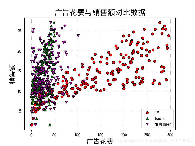
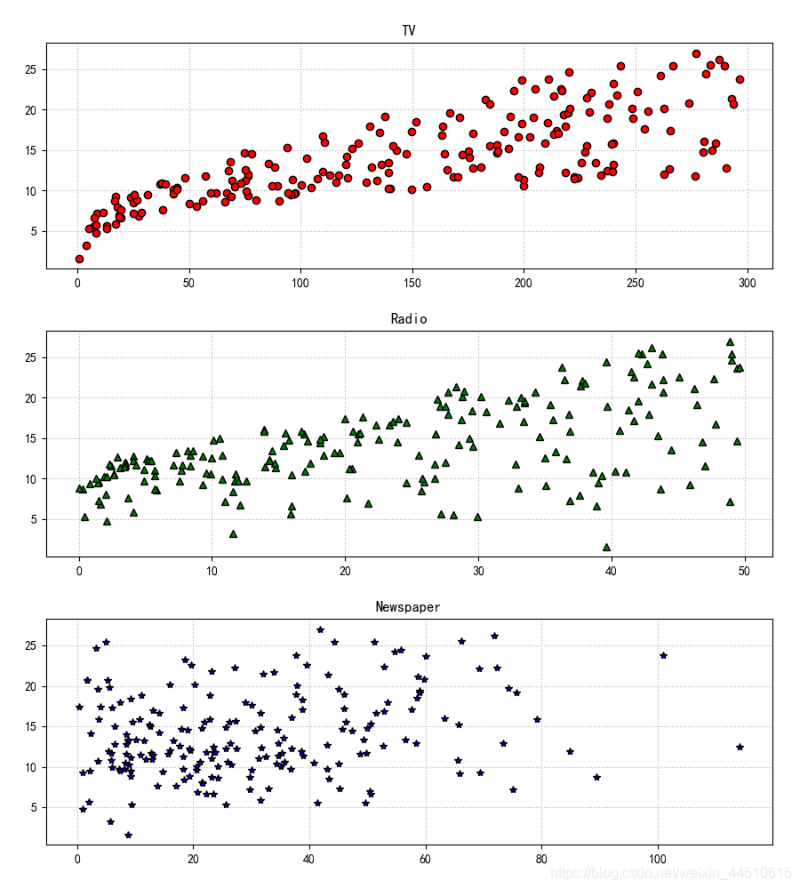
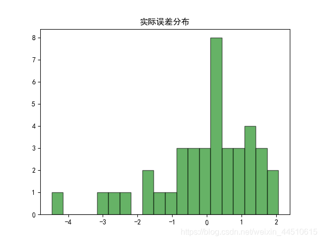
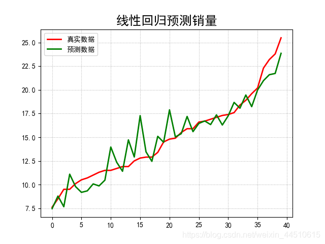
if __name__ == "__main__": show = False path = './Advertising.csv' # pandas读入 data = pd.read_csv(path) # TV、Radio、Newspaper、Sales x = data[['TV', 'Radio', 'Newspaper']] # x = data[['TV', 'Radio']] y = data['Sales'] print('Persone Corr = \n', data.corr()) # print(x) # print(y) # print(x.shape, y.shape) mpl.rcParams['font.sans-serif'] = ['simHei'] mpl.rcParams['axes.unicode_minus'] = False # 绘制1  广告花费与销售额对比数据 plt.figure(facecolor='white') plt.plot(data['TV'], y, 'ro', label='TV', mec='k') plt.plot(data['Radio'], y, 'g^', mec='k', label='Radio') plt.plot(data['Newspaper'], y, 'mv', mec='k', label='Newspaer') plt.legend(loc='lower right') plt.xlabel('广告花费', fontsize=16) plt.ylabel('销售额', fontsize=16) plt.title('广告花费与销售额对比数据', fontsize=18) plt.grid(b=True, ls=':') plt.show() # 绘制2  各自点的分布 plt.figure(facecolor='w', figsize=(9, 10)) plt.subplot(311) plt.plot(data['TV'], y, 'ro', mec='k') plt.title('TV') plt.grid(b=True, ls=':') plt.subplot(312) plt.plot(data['Radio'], y, 'g^', mec='k') plt.title('Radio') plt.grid(b=True, ls=':') plt.subplot(313) plt.plot(data['Newspaper'], y, 'b*', mec='k') plt.title('Newspaper') plt.grid(b=True, ls=':') plt.tight_layout(pad=2) # plt.savefig('three_graph.png') plt.show() x_train, x_test, y_train, y_test = train_test_split(x, y, test_size=0.2, random_state=1) model = LinearRegression() model.fit(x_train, y_train) print(model.coef_, model.intercept_) order = y_test.argsort(axis=0) y_test = y_test.values[order] x_test = x_test.values[order, :] y_test_pred = model.predict(x_test) mse = np.mean((y_test_pred - np.array(y_test)) ** 2)  # Mean Squared Error rmse = np.sqrt(mse)  # Root Mean Squared Error mse_sys = mean_squared_error(y_test, y_test_pred) print('MSE = ', mse, end=' ') print('MSE(System Function) = ', mse_sys, end=' ') print('MAE = ', mean_absolute_error(y_test, y_test_pred)) print('RMSE = ', rmse) print('Training R2 = ', model.score(x_train, y_train)) print('Training R2(System) = ', r2_score(y_train, model.predict(x_train))) print('Test R2 = ', model.score(x_test, y_test)) error = y_test - y_test_pred np.set_printoptions(suppress=True) print('error = ', error) plt.hist(error, bins=20, color='g', alpha=0.6, edgecolor='k') plt.title('实际误差分布') plt.show() plt.figure(facecolor='w') t = np.arange(len(x_test)) plt.plot(t, y_test, 'r-', linewidth=2, label='真实数据') plt.plot(t, y_test_pred, 'g-', linewidth=2, label='预测数据') plt.legend(loc='upper left') plt.title('线性回归预测销量', fontsize=18) plt.grid(b=True, ls=':') plt.show()


  

 

  
1
  
2
  
3
  
4
  
5
  
6
  
7
  
8
  
9
  
10
  
11
  
12
  
13
  
14
  
15
  
16
  
17
  
18
  
19
  
20
  
21
  
22
  
23
  
24
  
25
  
26
  
27
  
28
  
29
  
30
  
31
  
32
  
33
  
34
  
35
  
36
  
37
  
38
  
39
  
40
  
41
  
42
  
43
  
44
  
45
  
46
  
47
  
48
  
49
  
50
  
51
  
52
  
53
  
54
  
55
  
56
  
57
  
58
  
59
  
60
  
61
  
62
  
63
  
64
  
65
  
66
  
67
  
68
  
69
  
70
  
71
  
72
  
73
  
74
  
75
  
76
  
77
  
78
  
79
  
80
  
81
  
82
  
83
  
84
  
85
  
86
  
87
  
88
  
89
  
90
  
91
  
92
  
93
  
94
  
95
  
96
 

文章来源: maoli.blog.csdn.net，作者：刘润森！，版权归原作者所有，如需转载，请联系作者。

原文链接：maoli.blog.csdn.net/article/details/89457055