自然语言处理美国政客的社交媒体消息分类

【摘要】 数据简介: Disasters on social media
美国政客的社交媒体消息分类 内容:收集了来自美国参议员和其他美国政客的数千条社交媒体消息,可按内容分类为目标群众(国家或选民)、政治主张(中立/两党或偏见/党派)和实际内容(如攻击政敌等)
社交媒体上有些讨论是关于灾难,疾病,暴乱的,有些只是开玩笑或者是电影情节,我们该如何让机器能分辨出这两种讨论呢? ...
数据简介: Disasters on social media
美国政客的社交媒体消息分类
内容:收集了来自美国参议员和其他美国政客的数千条社交媒体消息,可按内容分类为目标群众(国家或选民)、政治主张(中立/两党或偏见/党派)和实际内容(如攻击政敌等)
社交媒体上有些讨论是关于灾难,疾病,暴乱的,有些只是开玩笑或者是电影情节,我们该如何让机器能分辨出这两种讨论呢?
import keras
import nltk
import pandas as pd
import numpy as np
import re
import codecs
- 1
- 2
- 3
- 4
- 5
- 6
questions = pd.read_csv("socialmedia_relevant_cols_clean.csv")
questions.columns=['text', 'choose_one', 'class_label']
questions.head()
- 1
- 2
- 3
| text | choose_one | class_label | |
|---|---|---|---|
| 0 | Just happened a terrible car crash | Relevant | 1 |
| 1 | Our Deeds are the Reason of this #earthquake M... | Relevant | 1 |
| 2 | Heard about #earthquake is different cities, s... | Relevant | 1 |
| 3 | there is a forest fire at spot pond, geese are... | Relevant | 1 |
| 4 | Forest fire near La Ronge Sask. Canada | Relevant | 1 |
questions.describe()
- 1
| class_label | |
|---|---|
| count | 10876.000000 |
| mean | 0.432604 |
| std | 0.498420 |
| min | 0.000000 |
| 25% | 0.000000 |
| 50% | 0.000000 |
| 75% | 1.000000 |
| max | 2.000000 |
数据清洗,去掉无用字符
def standardize_text(df, text_field): df[text_field] = df[text_field].str.replace(r"http\S+", "") df[text_field] = df[text_field].str.replace(r"http", "") df[text_field] = df[text_field].str.replace(r"@\S+", "") df[text_field] = df[text_field].str.replace(r"[^A-Za-z0-9(),!?@\'\`\"\_\n]", " ") df[text_field] = df[text_field].str.replace(r"@", "at") df[text_field] = df[text_field].str.lower() return df

questions = standardize_text(questions, "text")

questions.to_csv("clean_data.csv")
questions.head()
- 1
- 2
- 3
- 4
- 5
- 6
- 7
- 8
- 9
- 10
- 11
- 12
- 13
| text | choose_one | class_label | |
|---|---|---|---|
| 0 | just happened a terrible car crash | Relevant | 1 |
| 1 | our deeds are the reason of this earthquake m... | Relevant | 1 |
| 2 | heard about earthquake is different cities, s... | Relevant | 1 |
| 3 | there is a forest fire at spot pond, geese are... | Relevant | 1 |
| 4 | forest fire near la ronge sask canada | Relevant | 1 |
clean_questions = pd.read_csv("clean_data.csv")
clean_questions.tail()
- 1
- 2
| Unnamed: 0 | text | choose_one | class_label | |
|---|---|---|---|---|
| 10871 | 10871 | m1 94 01 04 utc ?5km s of volcano hawaii | Relevant | 1 |
| 10872 | 10872 | police investigating after an e bike collided ... | Relevant | 1 |
| 10873 | 10873 | the latest more homes razed by northern calif... | Relevant | 1 |
| 10874 | 10874 | meg issues hazardous weather outlook (hwo) | Relevant | 1 |
| 10875 | 10875 | cityofcalgary has activated its municipal eme... | Relevant | 1 |
数据分布情况
数据是否倾斜
clean_questions.groupby("class_label").count()
- 1
| Unnamed: 0 | text | choose_one | |
|---|---|---|---|
| class_label | |||
| 0 | 6187 | 6187 | 6187 |
| 1 | 4673 | 4673 | 4673 |
| 2 | 16 | 16 | 16 |
看起来还算均衡的
处理流程
- 分词
- 训练与测试集
- 检查与验证
from nltk.tokenize import RegexpTokenizer

tokenizer = RegexpTokenizer(r'\w+')

clean_questions["tokens"] = clean_questions["text"].apply(tokenizer.tokenize)
clean_questions.head()
- 1
- 2
- 3
- 4
- 5
- 6
| Unnamed: 0 | text | choose_one | class_label | tokens | |
|---|---|---|---|---|---|
| 0 | 0 | just happened a terrible car crash | Relevant | 1 | [just, happened, a, terrible, car, crash] |
| 1 | 1 | our deeds are the reason of this earthquake m... | Relevant | 1 | [our, deeds, are, the, reason, of, this, earth... |
| 2 | 2 | heard about earthquake is different cities, s... | Relevant | 1 | [heard, about, earthquake, is, different, citi... |
| 3 | 3 | there is a forest fire at spot pond, geese are... | Relevant | 1 | [there, is, a, forest, fire, at, spot, pond, g... |
| 4 | 4 | forest fire near la ronge sask canada | Relevant | 1 | [forest, fire, near, la, ronge, sask, canada] |
语料库情况
from keras.preprocessing.text import Tokenizer
from keras.preprocessing.sequence import pad_sequences
from keras.utils import to_categorical

all_words = [word for tokens in clean_questions["tokens"] for word in tokens]
sentence_lengths = [len(tokens) for tokens in clean_questions["tokens"]]
VOCAB = sorted(list(set(all_words)))
print("%s words total, with a vocabulary size of %s" % (len(all_words), len(VOCAB)))
print("Max sentence length is %s" % max(sentence_lengths))
- 1
- 2
- 3
- 4
- 5
- 6
- 7
- 8
- 9
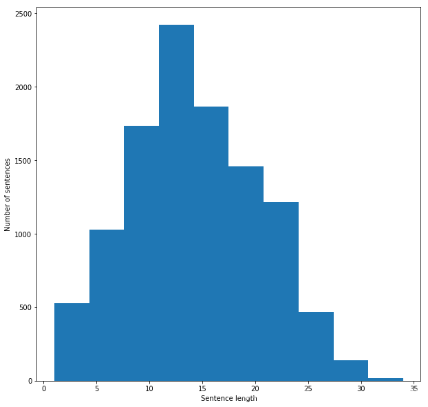
154724 words total, with a vocabulary size of 18101
Max sentence length is 34
- 1
- 2
句子长度情况
import matplotlib.pyplot as plt

fig = plt.figure(figsize=(10, 10))
plt.xlabel('Sentence length')
plt.ylabel('Number of sentences')
plt.hist(sentence_lengths)
plt.show()
- 1
- 2
- 3
- 4
- 5
- 6
- 7
特征如何构建?
Bag of Words Counts
from sklearn.model_selection import train_test_split
from sklearn.feature_extraction.text import CountVectorizer, TfidfVectorizer

def cv(data): count_vectorizer = CountVectorizer() emb = count_vectorizer.fit_transform(data) return emb, count_vectorizer

list_corpus = clean_questions["text"].tolist()
list_labels = clean_questions["class_label"].tolist()

X_train, X_test, y_train, y_test = train_test_split(list_corpus, list_labels, test_size=0.2, random_state=40)

X_train_counts, count_vectorizer = cv(X_train)
X_test_counts = count_vectorizer.transform(X_test)
- 1
- 2
- 3
- 4
- 5
- 6
- 7
- 8
- 9
- 10
- 11
- 12
- 13
- 14
- 15
- 16
- 17
- 18
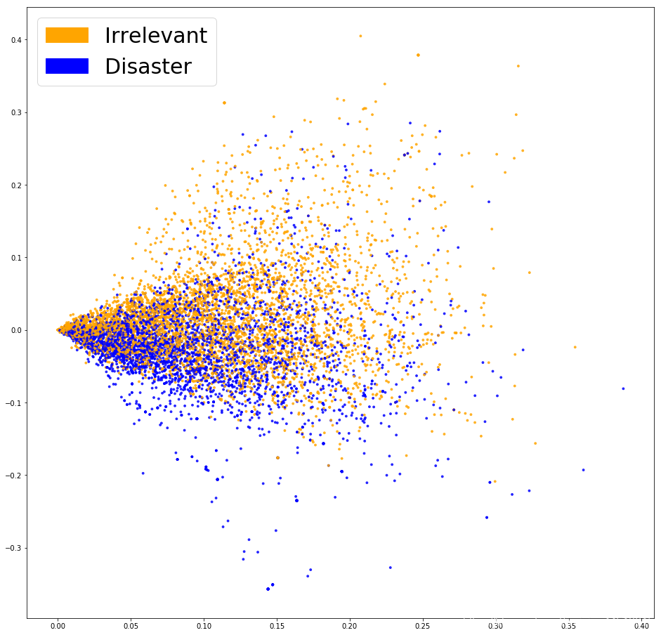
PCA展示Bag of Words
from sklearn.decomposition import PCA, TruncatedSVD
import matplotlib
import matplotlib.patches as mpatches


def plot_LSA(test_data, test_labels, savepath="PCA_demo.csv", plot=True): lsa = TruncatedSVD(n_components=2) lsa.fit(test_data) lsa_scores = lsa.transform(test_data) color_mapper = {label:idx for idx,label in enumerate(set(test_labels))} color_column = [color_mapper[label] for label in test_labels] colors = ['orange','blue','blue'] if plot: plt.scatter(lsa_scores[:,0], lsa_scores[:,1], s=8, alpha=.8, c=test_labels, cmap=matplotlib.colors.ListedColormap(colors)) red_patch = mpatches.Patch(color='orange', label='Irrelevant') green_patch = mpatches.Patch(color='blue', label='Disaster') plt.legend(handles=[red_patch, green_patch], prop={'size': 30})


fig = plt.figure(figsize=(16, 16)) plot_LSA(X_train_counts, y_train)
plt.show()
- 1
- 2
- 3
- 4
- 5
- 6
- 7
- 8
- 9
- 10
- 11
- 12
- 13
- 14
- 15
- 16
- 17
- 18
- 19
- 20
- 21
- 22
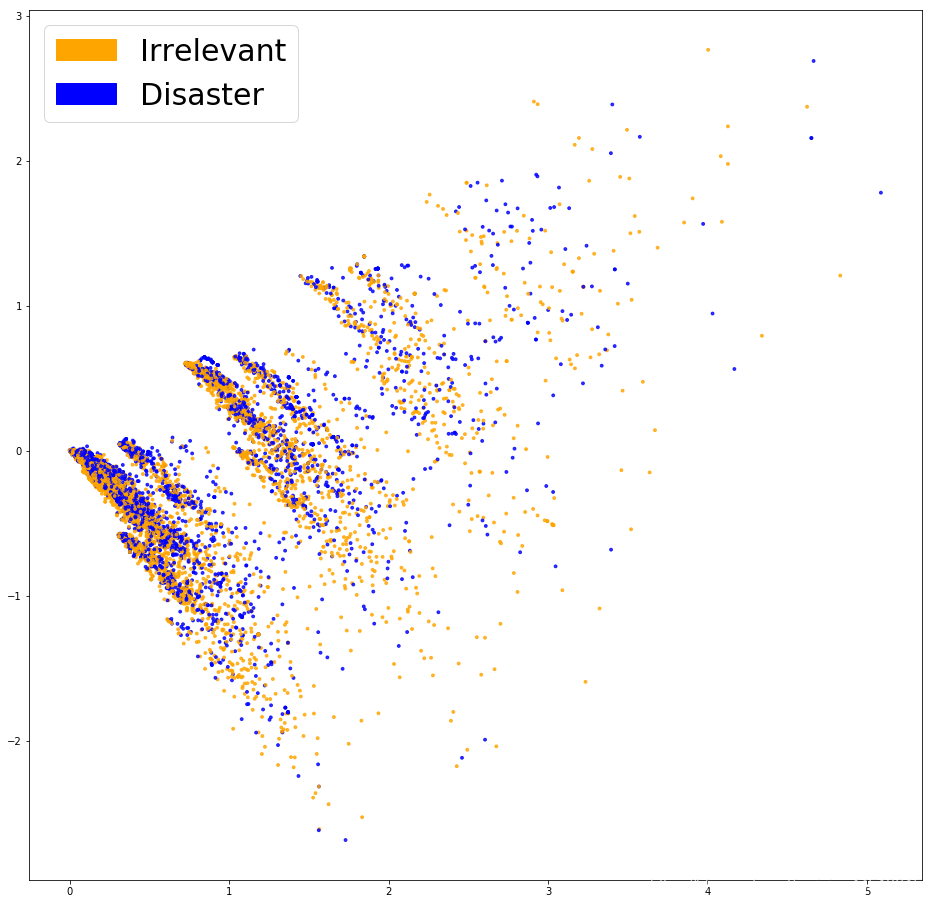
看起来并没有将这两类点区分开
逻辑回归看一下结果
from sklearn.linear_model import LogisticRegression

clf = LogisticRegression(C=30.0, class_weight='balanced', solver='newton-cg', multi_class='multinomial', n_jobs=-1, random_state=40)
clf.fit(X_train_counts, y_train)

y_predicted_counts = clf.predict(X_test_counts)
- 1
- 2
- 3
- 4
- 5
- 6
- 7
评估
from sklearn.metrics import accuracy_score, f1_score, precision_score, recall_score, classification_report

def get_metrics(y_test, y_predicted): # true positives / (true positives+false positives) precision = precision_score(y_test, y_predicted, pos_label=None, average='weighted') # true positives / (true positives + false negatives) recall = recall_score(y_test, y_predicted, pos_label=None, average='weighted') # harmonic mean of precision and recall f1 = f1_score(y_test, y_predicted, pos_label=None, average='weighted') # true positives + true negatives/ total accuracy = accuracy_score(y_test, y_predicted) return accuracy, precision, recall, f1

accuracy, precision, recall, f1 = get_metrics(y_test, y_predicted_counts)
print("accuracy = %.3f, precision = %.3f, recall = %.3f, f1 = %.3f" % (accuracy, precision, recall, f1))
- 1
- 2
- 3
- 4
- 5
- 6
- 7
- 8
- 9
- 10
- 11
- 12
- 13
- 14
- 15
- 16
- 17
- 18
- 19
accuracy = 0.754, precision = 0.752, recall = 0.754, f1 = 0.753
- 1
混淆矩阵检查
import numpy as np
import itertools
from sklearn.metrics import confusion_matrix

def plot_confusion_matrix(cm, classes, normalize=False, title='Confusion matrix', cmap=plt.cm.winter): if normalize: cm = cm.astype('float') / cm.sum(axis=1)[:, np.newaxis] plt.imshow(cm, interpolation='nearest', cmap=cmap) plt.title(title, fontsize=30) plt.colorbar() tick_marks = np.arange(len(classes)) plt.xticks(tick_marks, classes, fontsize=20) plt.yticks(tick_marks, classes, fontsize=20) fmt = '.2f' if normalize else 'd' thresh = cm.max() / 2. for i, j in itertools.product(range(cm.shape[0]), range(cm.shape[1])): plt.text(j, i, format(cm[i, j], fmt), horizontalalignment="center", color="white" if cm[i, j] < thresh else "black", fontsize=40) plt.tight_layout() plt.ylabel('True label', fontsize=30) plt.xlabel('Predicted label', fontsize=30) return plt
- 1
- 2
- 3
- 4
- 5
- 6
- 7
- 8
- 9
- 10
- 11
- 12
- 13
- 14
- 15
- 16
- 17
- 18
- 19
- 20
- 21
- 22
- 23
- 24
- 25
- 26
- 27
- 28
- 29
cm = confusion_matrix(y_test, y_predicted_counts)
fig = plt.figure(figsize=(10, 10))
plot = plot_confusion_matrix(cm, classes=['Irrelevant','Disaster','Unsure'], normalize=False, title='Confusion matrix')
plt.show()
print(cm)
- 1
- 2
- 3
- 4
- 5
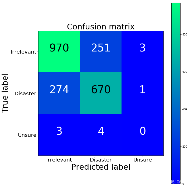
[[970 251   3]
 [274 670   1]
 [  3   4   0]]
- 1
- 2
- 3
第三类咋没有一个呢。。。因为数据里面就没几个啊。。。
进一步检查模型的关注点
def get_most_important_features(vectorizer, model, n=5): index_to_word = {v:k for k,v in vectorizer.vocabulary_.items()} # loop for each class classes ={} for class_index in range(model.coef_.shape[0]): word_importances = [(el, index_to_word[i]) for i,el in enumerate(model.coef_[class_index])] sorted_coeff = sorted(word_importances, key = lambda x : x[0], reverse=True) tops = sorted(sorted_coeff[:n], key = lambda x : x[0]) bottom = sorted_coeff[-n:] classes[class_index] = { 'tops':tops, 'bottom':bottom } return classes

importance = get_most_important_features(count_vectorizer, clf, 10)
- 1
- 2
- 3
- 4
- 5
- 6
- 7
- 8
- 9
- 10
- 11
- 12
- 13
- 14
- 15
- 16
- 17
def plot_important_words(top_scores, top_words, bottom_scores, bottom_words, name): y_pos = np.arange(len(top_words)) top_pairs = [(a,b) for a,b in zip(top_words, top_scores)] top_pairs = sorted(top_pairs, key=lambda x: x[1]) bottom_pairs = [(a,b) for a,b in zip(bottom_words, bottom_scores)] bottom_pairs = sorted(bottom_pairs, key=lambda x: x[1], reverse=True) top_words = [a[0] for a in top_pairs] top_scores = [a[1] for a in top_pairs] bottom_words = [a[0] for a in bottom_pairs] bottom_scores = [a[1] for a in bottom_pairs] fig = plt.figure(figsize=(10, 10)) plt.subplot(121) plt.barh(y_pos,bottom_scores, align='center', alpha=0.5) plt.title('Irrelevant', fontsize=20) plt.yticks(y_pos, bottom_words, fontsize=14) plt.suptitle('Key words', fontsize=16) plt.xlabel('Importance', fontsize=20) plt.subplot(122) plt.barh(y_pos,top_scores, align='center', alpha=0.5) plt.title('Disaster', fontsize=20) plt.yticks(y_pos, top_words, fontsize=14) plt.suptitle(name, fontsize=16) plt.xlabel('Importance', fontsize=20) plt.subplots_adjust(wspace=0.8) plt.show()

top_scores = [a[0] for a in importance[1]['tops']]
top_words = [a[1] for a in importance[1]['tops']]
bottom_scores = [a[0] for a in importance[1]['bottom']]
bottom_words = [a[1] for a in importance[1]['bottom']]

plot_important_words(top_scores, top_words, bottom_scores, bottom_words, "Most important words for relevance")
- 1
- 2
- 3
- 4
- 5
- 6
- 7
- 8
- 9
- 10
- 11
- 12
- 13
- 14
- 15
- 16
- 17
- 18
- 19
- 20
- 21
- 22
- 23
- 24
- 25
- 26
- 27
- 28
- 29
- 30
- 31
- 32
- 33
- 34
- 35
- 36
- 37
- 38
- 39
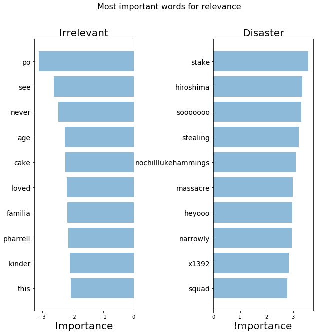
我们的模型找到了一些模式,但是看起来还不够好
TFIDF Bag of Words
这样我们就不均等对待每一个词了
def tfidf(data): tfidf_vectorizer = TfidfVectorizer() train = tfidf_vectorizer.fit_transform(data) return train, tfidf_vectorizer

X_train_tfidf, tfidf_vectorizer = tfidf(X_train)
X_test_tfidf = tfidf_vectorizer.transform(X_test)
- 1
- 2
- 3
- 4
- 5
- 6
- 7
- 8
- 9
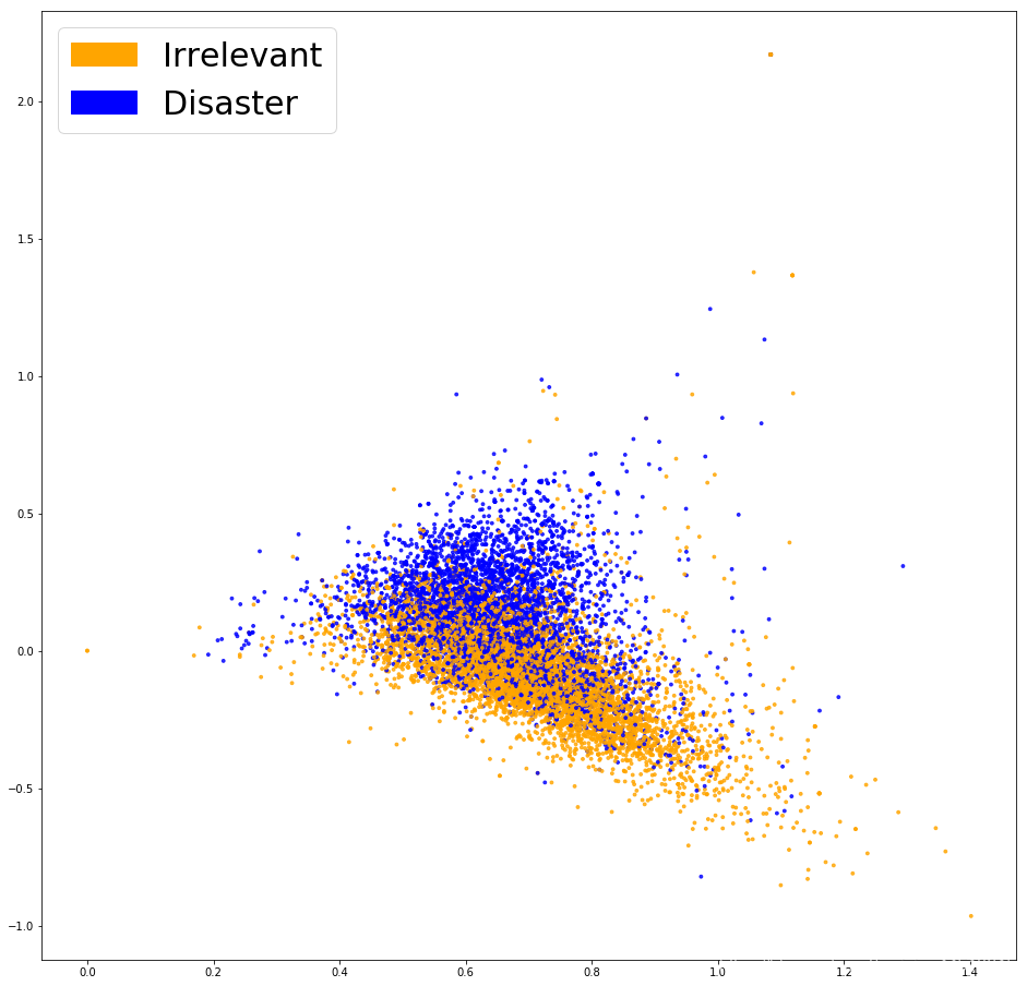
fig = plt.figure(figsize=(16, 16)) plot_LSA(X_train_tfidf, y_train)
plt.show()
- 1
- 2
- 3
看起来好那么一丁丁丁丁点
clf_tfidf = LogisticRegression(C=30.0, class_weight='balanced', solver='newton-cg', multi_class='multinomial', n_jobs=-1, random_state=40)
clf_tfidf.fit(X_train_tfidf, y_train)

y_predicted_tfidf = clf_tfidf.predict(X_test_tfidf)
- 1
- 2
- 3
- 4
- 5
accuracy_tfidf, precision_tfidf, recall_tfidf, f1_tfidf = get_metrics(y_test, y_predicted_tfidf)
print("accuracy = %.3f, precision = %.3f, recall = %.3f, f1 = %.3f" % (accuracy_tfidf, precision_tfidf, recall_tfidf, f1_tfidf))
- 1
- 2
- 3
accuracy = 0.762, precision = 0.760, recall = 0.762, f1 = 0.761
- 1
cm2 = confusion_matrix(y_test, y_predicted_tfidf)
fig = plt.figure(figsize=(10, 10))
plot = plot_confusion_matrix(cm2, classes=['Irrelevant','Disaster','Unsure'], normalize=False, title='Confusion matrix')
plt.show()
print("TFIDF confusion matrix")
print(cm2)
print("BoW confusion matrix")
print(cm)
- 1
- 2
- 3
- 4
- 5
- 6
- 7
- 8
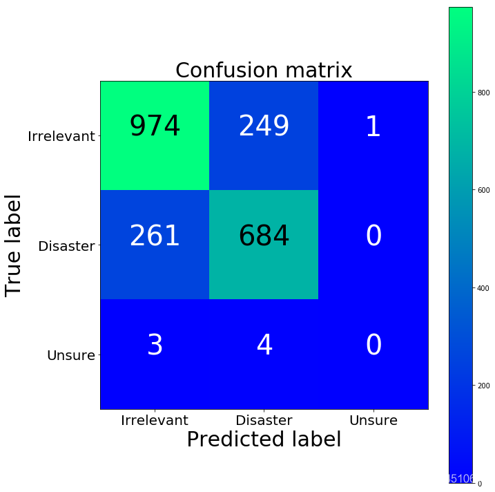
TFIDF confusion matrix
[[974 249   1]
 [261 684   0]
 [  3   4   0]]
BoW confusion matrix
[[970 251   3]
 [274 670   1]
 [  3   4   0]]
- 1
- 2
- 3
- 4
- 5
- 6
- 7
- 8
词语的解释
importance_tfidf = get_most_important_features(tfidf_vectorizer, clf_tfidf, 10)
- 1
top_scores = [a[0] for a in importance_tfidf[1]['tops']]
top_words = [a[1] for a in importance_tfidf[1]['tops']]
bottom_scores = [a[0] for a in importance_tfidf[1]['bottom']]
bottom_words = [a[1] for a in importance_tfidf[1]['bottom']]

plot_important_words(top_scores, top_words, bottom_scores, bottom_words, "Most important words for relevance")
- 1
- 2
- 3
- 4
- 5
- 6
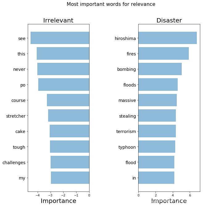
这些词看起来比之前强一些了
问题
我们现在考虑的是每一个词基于频率的情况,如果在新的测试环境下有些词变了呢?比如说goog和positive.有些词可能表达的意义差不多但是却长得不一样,这样我们的模型就难捕捉到了。
word2vec
一句话解释:比较牛逼。。。
import gensim

word2vec_path = "GoogleNews-vectors-negative300.bin"
word2vec = gensim.models.KeyedVectors.load_word2vec_format(word2vec_path, binary=True)
- 1
- 2
- 3
- 4
def get_average_word2vec(tokens_list, vector, generate_missing=False, k=300): if len(tokens_list)<1: return np.zeros(k) if generate_missing: vectorized = [vector[word] if word in vector else np.random.rand(k) for word in tokens_list] else: vectorized = [vector[word] if word in vector else np.zeros(k) for word in tokens_list] length = len(vectorized) summed = np.sum(vectorized, axis=0) averaged = np.divide(summed, length) return averaged

def get_word2vec_embeddings(vectors, clean_questions, generate_missing=False): embeddings = clean_questions['tokens'].apply(lambda x: get_average_word2vec(x, vectors, generate_missing=generate_missing)) return list(embeddings)
- 1
- 2
- 3
- 4
- 5
- 6
- 7
- 8
- 9
- 10
- 11
- 12
- 13
- 14
- 15
- 16
embeddings = get_word2vec_embeddings(word2vec, clean_questions)
X_train_word2vec, X_test_word2vec, y_train_word2vec, y_test_word2vec = train_test_split(embeddings, list_labels, test_size=0.2, random_state=40)
- 1
- 2
- 3
X_train_word2vec[0]
- 1
array([ 0.05639939, 0.02053833, 0.07635207, 0.06914993, -0.01007262, -0.04978943, 0.02546038, -0.06045968, 0.04264323, 0.02419935, 0.00375076, -0.15124639, 0.02915809, -0.01554943, -0.10182699, 0.05523972, 0.00953747, 0.0834525 , 0.00200544, -0.0238909 , -0.01706369, 0.09193638, 0.03979783, 0.04899052, 0.04707618, -0.09235491, -0.10698809, 0.07503255, 0.04905628, -0.01991781, 0.04036749, -0.0117856 , -0.00576346, 0.01624843, -0.01823952, -0.01545715, 0.06020392, 0.02975609, 0.02211217, 0.07844525, 0.05023847, -0.09430913, 0.20582217, -0.05274091, 0.00881231, 0.04394059, -0.01748512, -0.0403268 , 0.03178769, 0.06038993, 0.03867458, 0.00492932, 0.05121649, 0.01256743, -0.02096994, 0.02814593, -0.06389218, 0.01661319, -0.02686709, -0.07981364, -0.00288318, 0.07032367, -0.07524182, -0.01155599, -0.0259661 , 0.00625901, -0.05474758, -0.00059877, -0.01737177, 0.07586161, 0.0273136 , -0.00077093, 0.0752638 , 0.05861119, -0.15668742, -0.00779506, 0.04997617, 0.08768209, 0.04078311, 0.07749503, 0.02886018, -0.08094715, 0.05818976, -0.02744593, -0.00559489, -0.00488863, -0.06092762, 0.15089634, -0.02423968, 0.02867635, 0.0041097 , 0.00409226, -0.05106317, -0.0156715 , -0.06731596, 0.00594657, 0.02464658, 0.10740153, 0.0207287 , -0.02535357, -0.05631002, -0.01714507, -0.04964483, -0.00834728, -0.01148841, 0.04122198, 0.00281052, -0.02053833, 0.01521229, -0.10191563, -0.07321421, -0.01803589, -0.02788144, 0.00172424, 0.07978603, -0.01517505, 0.03893743, -0.0548212 , 0.03782436, 0.04642305, -0.05222284, 0.01304263, -0.06944965, 0.01763625, -0.02670433, -0.03698331, -0.02478899, -0.06544131, 0.05864679, -0.00175549, -0.11564055, -0.10066441, -0.04190209, -0.02992467, -0.08564534, -0.02061244, 0.02688017, -0.0045171 , 0.00165086, 0.10750544, -0.028361 , -0.03209577, 0.0515936 , -0.04164342, 0.02281843, 0.08524286, -0.10112653, -0.14161319, -0.05427769, -0.01017171, 0.09955125, 0.02694847, -0.0915055 , 0.09549531, -0.0138172 , 0.01547096, 0.00868443, -0.04557078, -0.00442069, 0.01043919, -0.00775728, 0.02804129, 0.10577102, 0.07417879, -0.0414545 , -0.10446894, 0.07996532, -0.06722441, 0.0636742 , -0.05054583, -0.11369978, 0.02922131, -0.03643508, -0.09067681, -0.06278338, -0.01135545, 0.09446498, -0.02156576, 0.00918143, 0.0722787 , -0.01088969, 0.03180022, -0.00304031, 0.0532895 , 0.07494827, -0.02797735, -0.06948853, 0.06283715, 0.10689872, 0.02087112, 0.05185082, 0.06266276, 0.01831927, 0.10564604, 0.00259254, 0.08089193, -0.01426479, 0.00684974, -0.03707304, -0.1198062 , -0.05715216, 0.01687549, 0.03455462, -0.08835565, 0.05120559, -0.06600516, -0.01664807, -0.02856736, 0.02654157, -0.00975818, -0.03065236, -0.04041981, -0.01071312, -0.05153402, -0.14723714, -0.00877744, 0.08035714, 0.00351824, -0.10722714, -0.03078206, -0.00496383, -0.01665388, 0.0004069 , -0.02276175, 0.14360192, -0.09488932, 0.00554548, 0.13301958, -0.02263096, -0.03730701, 0.03650629, -0.02395339, 0.00687372, -0.02563804, 0.03732518, -0.02720424, -0.0106114 , -0.05050805, 0.00444685, -0.02968924, 0.07124983, -0.00694057, 0.00107829, -0.08331589, -0.03359186, 0.0081293 , -0.0008138 , 0.01801554, 0.02518827, -0.03804089, 0.06714594, 0.00194731, 0.08901033, 0.06102903, 0.03237479, -0.05186026, 0.02203078, -0.02689325, -0.01497105, -0.07096935, 0.00406174, 0.03199695, -0.05650693, -0.00124395, 0.08180745, 0.10938081, 0.0316787 , 0.01944987, -0.02388909, 0.00355748, 0.0249256 , 0.00739524, 0.0506243 , -0.01226516, 0.01143035, -0.09211658, -0.02129836, -0.11622447, -0.04239509, -0.05391511, -0.00467064, -0.01021031, 0.00030227, 0.12456985, -0.0130964 , 0.02393832, -0.04647537, 0.06130255, 0.02752686, 0.04820469, -0.06352307, 0.0357637 , -0.1455921 , 0.01995268, -0.04385739, -0.03136626, -0.04338237, -0.08235096, 0.02723331, -0.01401483])
- 1
- 2
- 3
- 4
- 5
- 6
- 7
- 8
- 9
- 10
- 11
- 12
- 13
- 14
- 15
- 16
- 17
- 18
- 19
- 20
- 21
- 22
- 23
- 24
- 25
- 26
- 27
- 28
- 29
- 30
- 31
- 32
- 33
- 34
- 35
- 36
- 37
- 38
- 39
- 40
- 41
- 42
- 43
- 44
- 45
- 46
- 47
- 48
- 49
- 50
- 51
- 52
- 53
- 54
- 55
- 56
- 57
- 58
- 59
- 60
fig = plt.figure(figsize=(16, 16)) plot_LSA(embeddings, list_labels)
plt.show()
- 1
- 2
- 3
这看起来就好多啦!
clf_w2v = LogisticRegression(C=30.0, class_weight='balanced', solver='newton-cg', multi_class='multinomial', random_state=40)
clf_w2v.fit(X_train_word2vec, y_train_word2vec)
y_predicted_word2vec = clf_w2v.predict(X_test_word2vec)
- 1
- 2
- 3
- 4
accuracy_word2vec, precision_word2vec, recall_word2vec, f1_word2vec = get_metrics(y_test_word2vec, y_predicted_word2vec)
print("accuracy = %.3f, precision = %.3f, recall = %.3f, f1 = %.3f" % (accuracy_word2vec, precision_word2vec, recall_word2vec, f1_word2vec))
- 1
- 2
- 3
accuracy = 0.777, precision = 0.776, recall = 0.777, f1 = 0.777
- 1
cm_w2v = confusion_matrix(y_test_word2vec, y_predicted_word2vec)
fig = plt.figure(figsize=(10, 10))
plot = plot_confusion_matrix(cm, classes=['Irrelevant','Disaster','Unsure'], normalize=False, title='Confusion matrix')
plt.show()
print("Word2Vec confusion matrix")
print(cm_w2v)
print("TFIDF confusion matrix")
print(cm2)
print("BoW confusion matrix")
print(cm)
- 1
- 2
- 3
- 4
- 5
- 6
- 7
- 8
- 9
- 10

Word2Vec confusion matrix
[[980 242   2]
 [232 711   2]
 [  2   5   0]]
TFIDF confusion matrix
[[974 249   1]
 [261 684   0]
 [  3   4   0]]
BoW confusion matrix
[[970 251   3]
 [274 670   1]
 [  3   4   0]]
- 1
- 2
- 3
- 4
- 5
- 6
- 7
- 8
- 9
- 10
- 11
- 12
这是目前为止最好的啦
基于深度学习的自然语言处理(CNN与RNN)
from keras.preprocessing.text import Tokenizer
from keras.preprocessing.sequence import pad_sequences
from keras.utils import to_categorical

EMBEDDING_DIM = 300
MAX_SEQUENCE_LENGTH = 35
VOCAB_SIZE = len(VOCAB)

VALIDATION_SPLIT=.2
tokenizer = Tokenizer(num_words=VOCAB_SIZE)
tokenizer.fit_on_texts(clean_questions["text"].tolist())
sequences = tokenizer.texts_to_sequences(clean_questions["text"].tolist())

word_index = tokenizer.word_index
print('Found %s unique tokens.' % len(word_index))

cnn_data = pad_sequences(sequences, maxlen=MAX_SEQUENCE_LENGTH)
labels = to_categorical(np.asarray(clean_questions["class_label"]))

indices = np.arange(cnn_data.shape[0])
np.random.shuffle(indices)
cnn_data = cnn_data[indices]
labels = labels[indices]
num_validation_samples = int(VALIDATION_SPLIT * cnn_data.shape[0])

embedding_weights = np.zeros((len(word_index)+1, EMBEDDING_DIM))
for word,index in word_index.items(): embedding_weights[index,:] = word2vec[word] if word in word2vec else np.random.rand(EMBEDDING_DIM)
print(embedding_weights.shape)
- 1
- 2
- 3
- 4
- 5
- 6
- 7
- 8
- 9
- 10
- 11
- 12
- 13
- 14
- 15
- 16
- 17
- 18
- 19
- 20
- 21
- 22
- 23
- 24
- 25
- 26
- 27
- 28
- 29
Found 19098 unique tokens.
(19099, 300)
- 1
- 2
Now, we will define a simple Convolutional Neural Network
from keras.layers import Dense, Input, Flatten, Dropout, Merge
from keras.layers import Conv1D, MaxPooling1D, Embedding
from keras.layers import LSTM, Bidirectional
from keras.models import Model

def ConvNet(embeddings, max_sequence_length, num_words, embedding_dim, labels_index, trainable=False, extra_conv=True): embedding_layer = Embedding(num_words, embedding_dim, weights=[embeddings], input_length=max_sequence_length, trainable=trainable) sequence_input = Input(shape=(max_sequence_length,), dtype='int32') embedded_sequences = embedding_layer(sequence_input) # Yoon Kim model (https://arxiv.org/abs/1408.5882) convs = [] filter_sizes = [3,4,5] for filter_size in filter_sizes: l_conv = Conv1D(filters=128, kernel_size=filter_size, activation='relu')(embedded_sequences) l_pool = MaxPooling1D(pool_size=3)(l_conv) convs.append(l_pool) l_merge = Merge(mode='concat', concat_axis=1)(convs) # add a 1D convnet with global maxpooling, instead of Yoon Kim model conv = Conv1D(filters=128, kernel_size=3, activation='relu')(embedded_sequences) pool = MaxPooling1D(pool_size=3)(conv) if extra_conv==True: x = Dropout(0.5)(l_merge) else: # Original Yoon Kim model x = Dropout(0.5)(pool) x = Flatten()(x) x = Dense(128, activation='relu')(x) #x = Dropout(0.5)(x) preds = Dense(labels_index, activation='softmax')(x) model = Model(sequence_input, preds) model.compile(loss='categorical_crossentropy', optimizer='adam', metrics=['acc']) return model
- 1
- 2
- 3
- 4
- 5
- 6
- 7
- 8
- 9
- 10
- 11
- 12
- 13
- 14
- 15
- 16
- 17
- 18
- 19
- 20
- 21
- 22
- 23
- 24
- 25
- 26
- 27
- 28
- 29
- 30
- 31
- 32
- 33
- 34
- 35
- 36
- 37
- 38
- 39
- 40
- 41
- 42
- 43
- 44
- 45
- 46
- 47
- 48
训练网络
x_train = cnn_data[:-num_validation_samples]
y_train = labels[:-num_validation_samples]
x_val = cnn_data[-num_validation_samples:]
y_val = labels[-num_validation_samples:]

model = ConvNet(embedding_weights, MAX_SEQUENCE_LENGTH, len(word_index)+1, EMBEDDING_DIM, len(list(clean_questions["class_label"].unique())), False)
- 1
- 2
- 3
- 4
- 5
- 6
- 7
model.fit(x_train, y_train, validation_data=(x_val, y_val), epochs=3, batch_size=128)
- 1
Train on 8701 samples, validate on 2175 samples
Epoch 1/3
8701/8701 [==============================] - 11s - loss: 0.5964 - acc: 0.7067 - val_loss: 0.4970 - val_acc: 0.7848
Epoch 2/3
8701/8701 [==============================] - 11s - loss: 0.4434 - acc: 0.8019 - val_loss: 0.4722 - val_acc: 0.8005
Epoch 3/3
8701/8701 [==============================] - 11s - loss: 0.3968 - acc: 0.8283 - val_loss: 0.4985 - val_acc: 0.7880
<keras.callbacks.History at 0x12237bc88>
- 1
- 2
- 3
- 4
- 5
- 6
- 7
- 8
文章来源: maoli.blog.csdn.net,作者:刘润森!,版权归原作者所有,如需转载,请联系作者。
原文链接:maoli.blog.csdn.net/article/details/89842983

【版权声明】本文为华为云社区用户转载文章,如果您发现本社区中有涉嫌抄袭的内容,欢迎发送邮件进行举报,并提供相关证据,一经查实,本社区将立刻删除涉嫌侵权内容,举报邮箱:
cloudbbs@huaweicloud.com
- 点赞
- 收藏
- 关注作者
评论(0)