浅谈目标检测中常规的回归loss计算----------最新yolov4中ciou计算

前言
今天我们来看下目标检测里面提出的CIOU。
目标检测loss的发展史
在目标检测中其演进路线是Smooth L1 Loss --> IoU Loss --> GIoU Loss --> DIoU Loss --.>CIoU Loss
学习前言
什么是iou
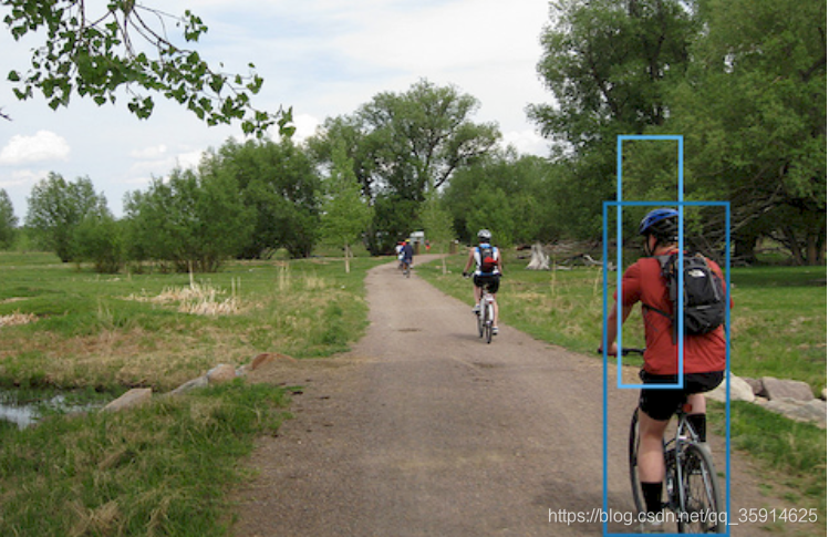
Intersection over Union (IoU) 是目标检测里一种重要的评价值。上面第一张途中框出了 gt box 和 predict box,IoU 通过计算这两个框 A、B 间的 Intersection Area I(相交的面积) 和 Union Area U(总的面积) 的比值来获得

什么是Smooth L1 Loss?
首先看L1 loss 和 L2 loss 定义:
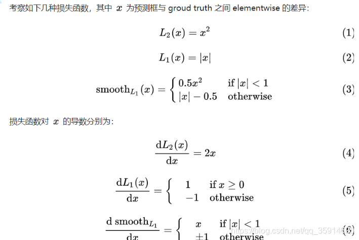
写成差的形式,f(x) 为预测值, Y 为 groud truth

对于L2 Loss:当 x 增大时 L2 损失对 x 的导数也增大。这就导致训练初期,预测值与 groud truth 差异过于大时,损失函数对预测值的梯度十分大,训练不稳定。从下面的形式 L2 Loss的梯度包含 (f(x) - Y),当预测值 f(x) 与目标值 Y 相差很大时(此时可能是离群点、异常值(outliers)),容易产生梯度爆炸
对于L1 Loss:根据方程 (5),L1 对 x 的导数为常数。这就导致训练后期,预测值与 ground truth 差异很小时, L1 损失对预测值的导数的绝对值仍然为 1,而 learning rate 如果不变,损失函数将在稳定值附近波动,难以继续收敛以达到更高精度。
从上面的导数可以看出,L2 Loss的梯度包含 (f(x) - Y),当预测值 f(x) 与目标值 Y 相差很大时,容易产生梯度爆炸。在L1 Loss时的梯度为常数。通过使用Smooth L1 Loss,在预测值与目标值相差较大时,由L2 Loss转为L1 Loss可以防止梯度爆炸。
Smooth L1 Loss 完美的避开了 L1和 L2损失的缺点。

实际目标检测框回归任务中的损失loss为 :

其中
表示GT 的框坐标,

表示预测的框坐标,即分别求4个点的loss,然后相加作为Bounding Box Regression Loss。
缺点
1.上面的三种Loss用于计算目标检测的Bounding Box Loss时,独立的求出4个点的Loss,然后进行相加得到最终的Bounding Box Loss,这种做法的假设是4个点是相互独立的,实际是有一定相关性的
2.实际评价框检测的指标是使用IOU,这两者是不等价的,多个检测框可能有相同大小的smooth Loss,但IOU可能差异很大,为了解决这个问题就引入了IOU LOSS。
代码:
def smooth_l1(sigma=1.0): sigma_squared = sigma ** 2 def _smooth_l1(y_true, y_pred): # y_true [batch_size, num_anchor, 4+1] # y_pred [batch_size, num_anchor, 4] regression = y_pred regression_target = y_true[:, :, :-1] anchor_state = y_true[:, :, -1] # 找到正样本 indices = tf.where(keras.backend.equal(anchor_state, 1)) regression = tf.gather_nd(regression, indices) regression_target = tf.gather_nd(regression_target, indices) # 计算 smooth L1 loss # f(x) = 0.5 * (sigma * x)^2 if |x| < 1 / sigma / sigma # |x| - 0.5 / sigma / sigma otherwise #keras.backend.less逐个元素比对 (x < y) 的真值。
#参数:

#x:张量或变量。
#y:张量或变量。 regression_diff = regression - regression_target regression_diff = keras.backend.abs(regression_diff) regression_loss = tf.where( keras.backend.less(regression_diff, 1.0 / sigma_squared), 0.5 * sigma_squared * keras.backend.pow(regression_diff, 2), regression_diff - 0.5 / sigma_squared ) normalizer = keras.backend.maximum(1, keras.backend.shape(indices)[0]) normalizer = keras.backend.cast(normalizer, dtype=keras.backend.floatx()) loss = keras.backend.sum(regression_loss) / normalizer return loss return _smooth_l
- 1
- 2
- 3
- 4
- 5
- 6
- 7
- 8
- 9
- 10
- 11
- 12
- 13
- 14
- 15
- 16
- 17
- 18
- 19
- 20
- 21
- 22
- 23
- 24
- 25
- 26
- 27
- 28
- 29
- 30
- 31
- 32
- 33
- 34
- 35
- 36
- 37
- 38
什么是IoU Loss?

图中第一行,所有目标的L1 Loss都一样,但是第三个的IOU显然是要大于第一个,并且第3个的检测结果似乎也是好于第一个的。第二行类似,所有目标的L1 Loss也都一样,但IOU却存在差异。因此使用bbox和ground truth bbox的L1范数,L2范数来计算位置回归Loss以及在评测的时候却使用IOU(交并比)去判断是否检测到目标是有一个界限的,这两者并不等价。
基于此提出IoU Loss,其将4个点构成的box看成一个整体进行回归:
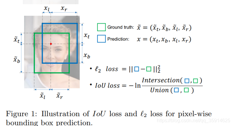
上图展示了L2 Loss和IoU Loss 的求法,图中红点表示目标检测网络结构中Head部分上的点(i,j),绿色的框表示GT框, 蓝色的框表示Prediction的框。
IoU loss的定义如上,先求出2个框的IoU,然后再求个**-ln(IoU),在实际使用中,实际很多IoU常常被定义为IoU Loss = 1-IoU。**
其中IoU是真实框和预测框的交集和并集之比,当它们完全重合时,IoU就是1,那么对于Loss来说,Loss是越小越好,说明他们重合度高,所以IoU Loss就可以简单表示为 1- IoU。
缺点:
1.预测框bbox和ground truth bbox如果没有重叠,IOU就始终为0并且无法优化。也就是说损失函数失去了可导的性质。
2.IOU无法分辨不同方式的对齐,例如方向不一致等,如下图所示,可以看到三种方式拥有相同的IOU值,但空间方向却完全不同,IoU值不能反映两个框是如何相交的。

import numpy as np
def Iou(box1, box2, wh=False): if wh == False:
	xmin1, ymin1, xmax1, ymax1 = box1
	xmin2, ymin2, xmax2, ymax2 = box2 else:
	xmin1, ymin1 = int(box1[0]-box1[2]/2.0), int(box1[1]-box1[3]/2.0)
	xmax1, ymax1 = int(box1[0]+box1[2]/2.0), int(box1[1]+box1[3]/2.0)
	xmin2, ymin2 = int(box2[0]-box2[2]/2.0), int(box2[1]-box2[3]/2.0)
	xmax2, ymax2 = int(box2[0]+box2[2]/2.0), int(box2[1]+box2[3]/2.0) # 获取矩形框交集对应的左上角和右下角的坐标(intersection) xx1 = np.max([xmin1, xmin2]) yy1 = np.max([ymin1, ymin2]) xx2 = np.min([xmax1, xmax2]) yy2 = np.min([ymax1, ymax2]) # 计算两个矩形框面积 area1 = (xmax1-xmin1) * (ymax1-ymin1) area2 = (xmax2-xmin2) * (ymax2-ymin2) inter_area = (np.max([0, xx2-xx1])) * (np.max([0, yy2-yy1])) #计算交集面积 iou = inter_area / (area1+area2-inter_area+1e-6)  #计算交并比 return iou
- 1
- 2
- 3
- 4
- 5
- 6
- 7
- 8
- 9
- 10
- 11
- 12
- 13
- 14
- 15
- 16
- 17
- 18
- 19
- 20
- 21
- 22
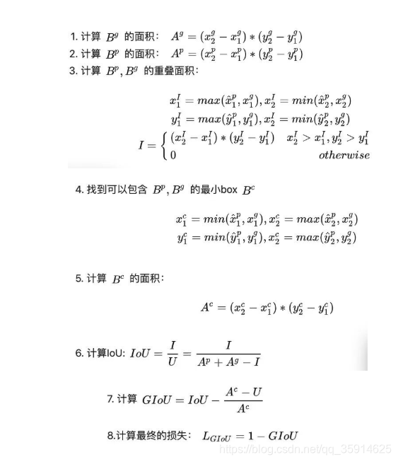
什么是GIoU Loss?
GIoU 作为 IoU 的升级版,既继承了 IoU 的两个优点,又弥补了 IoU 无法衡量无重叠框之间的距离的缺点。具体计算方式是在 IoU 计算的基础上寻找一个 smallest convex shapes C。那么他是怎样设计的?
假如现在有两个任意性质 A,B,我们找到一个最小的封闭形状C,让C可以把A,B包含在内,然后我们计算C中没有覆盖A和B的面积占C总面积的比值,然后用A与B的IoU减去这个比值:

GIoU有如下性质:
与IoU类似,GIoU也可以作为一个距离,loss可以用 (下面的公式)来计算:
-1<=GIoU<=1,当A=B时,GIoU=IoU=1;当A与B不相交而且离得很远时,GIoU(A,B)趋向于-1。loss=1-GIoU。
具体一点,如何计算损失呢?
假设我们现在有预测的 Bbox 和 groud truth 的 Bbox 的坐标,分别记为:

注意我们规定对于预测的 BBox 来说,有

主要是为了方便之后点的对应关系。
def Giou(rec1,rec2): #分别是第一个矩形左右上下的坐标 x1,x2,y1,y2 = rec1 x3,x4,y3,y4 = rec2 iou = Iou(rec1,rec2) area_C = (max(x1,x2,x3,x4)-min(x1,x2,x3,x4))*(max(y1,y2,y3,y4)-min(y1,y2,y3,y4)) area_1 = (x2-x1)*(y1-y2) area_2 = (x4-x3)*(y3-y4) sum_area = area_1 + area_2 w1 = x2 - x1 #第一个矩形的宽 w2 = x4 - x3 #第二个矩形的宽 h1 = y1 - y2 h2 = y3 - y4 W = min(x1,x2,x3,x4)+w1+w2-max(x1,x2,x3,x4) #交叉部分的宽 H = min(y1,y2,y3,y4)+h1+h2-max(y1,y2,y3,y4) #交叉部分的高 Area = W*H #交叉的面积 add_area = sum_area - Area #两矩形并集的面积 end_area = (area_C - add_area)/area_C #闭包区域中不属于两个框的区域占闭包区域的比重 giou = iou - end_area return giou
- 1
- 2
- 3
- 4
- 5
- 6
- 7
- 8
- 9
- 10
- 11
- 12
- 13
- 14
- 15
- 16
- 17
- 18
- 19
- 20
- 21
- 22
缺点:
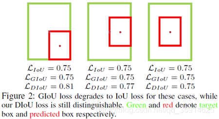
当目标框完全包裹预测框的时候,IoU和GIoU的值都一样,此时GIoU退化为IoU, 无法区分其相对位置关系。
什么是DIoU Loss?
基于IoU和GIoU存在的问题,作者提出了两个问题:
第一:直接最小化预测框与目标框之间的归一化距离是否可行,以达到更快的收敛速度。
第二:如何使回归在与目标框有重叠甚至包含时更准确、更快。
好的目标框回归损失应该考虑三个重要的几何因素:重叠面积,中心点距离,长宽比。基于问题一,作者提出了DIoU Loss,相对于GIoU Loss收敛速度更快,该Loss考虑了重叠面积和中心点距离,但没有考虑到长宽比;针对问题二,作者提出了CIoU Loss,其收敛的精度更高,以上三个因素都考虑到了。
针对**直接最小化Anchor和目标框之间的归一化距离以达到更快的收敛速度是否可行?**提出了Distance-IoU Loss(DIoU Loss)。
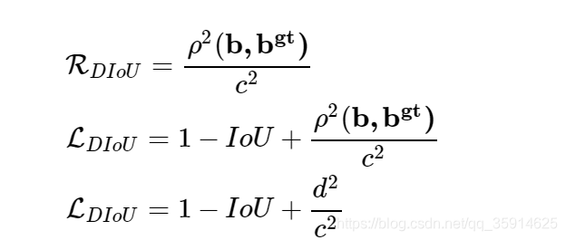
这个损失函数中,b,bgt分别代表了Anchor框和目标框的中心点,p代表计算两个中心点的欧式距离,c代表的是可以同时覆盖Anchor框和目标框的最小矩形的对角线距离。因此DIoU中对Anchor框和目标框之间的归一化距离进行了建模。直观展如下图
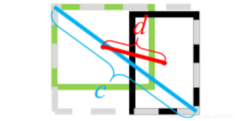
上图中绿色框为目标框,黑色框为预测框,灰色框为两者的最小外界矩形框,d表示目标框和真实框的中心点距离,c表示最小外界矩形框的距离。
优点:
1.与GIoU loss 类似,DIoU loss 在与目标框不重叠时,仍然可以为边界框提供移动方向。
2.DIoU loss 可以直接最小化两个目标框的距离,因此比 GIoU loss 收敛快得多。
3.对于包含两个框在水平方向和垂直方向上这种情况,DIoU loss 可以使回归非常快,而 GIoU loss 几乎退化为 IoU loss。
4.当两个框完全重合Ldlou=Llou=Lglou=0,当两个框完全不相交时Ldlou=LGiou->2
5.DIoU 还可以替换普通的 IoU 评价策略,应用于 NMS 中,使得 NMS 得到的结果更加合理和有效。
代码:
def Diou(bboxes1, bboxes2): rows = bboxes1.shape[0] cols = bboxes2.shape[0] dious = torch.zeros((rows, cols)) if rows * cols == 0:# return dious exchange = False if bboxes1.shape[0] > bboxes2.shape[0]: bboxes1, bboxes2 = bboxes2, bboxes1 dious = torch.zeros((cols, rows)) exchange = True # #xmin,ymin,xmax,ymax->[:,0],[:,1],[:,2],[:,3] w1 = bboxes1[:, 2] - bboxes1[:, 0] h1 = bboxes1[:, 3] - bboxes1[:, 1] w2 = bboxes2[:, 2] - bboxes2[:, 0] h2 = bboxes2[:, 3] - bboxes2[:, 1] area1 = w1 * h1 area2 = w2 * h2 center_x1 = (bboxes1[:, 2] + bboxes1[:, 0]) / 2 center_y1 = (bboxes1[:, 3] + bboxes1[:, 1]) / 2 center_x2 = (bboxes2[:, 2] + bboxes2[:, 0]) / 2 center_y2 = (bboxes2[:, 3] + bboxes2[:, 1]) / 2 inter_max_xy = torch.min(bboxes1[:, 2:],bboxes2[:, 2:]) inter_min_xy = torch.max(bboxes1[:, :2],bboxes2[:, :2]) out_max_xy = torch.max(bboxes1[:, 2:],bboxes2[:, 2:]) out_min_xy = torch.min(bboxes1[:, :2],bboxes2[:, :2]) inter = torch.clamp((inter_max_xy - inter_min_xy), min=0) inter_area = inter[:, 0] * inter[:, 1] inter_diag = (center_x2 - center_x1)**2 + (center_y2 - center_y1)**2 outer = torch.clamp((out_max_xy - out_min_xy), min=0) outer_diag = (outer[:, 0] ** 2) + (outer[:, 1] ** 2) union = area1+area2-inter_area dious = inter_area / union - (inter_diag) / outer_diag dious = torch.clamp(dious,min=-1.0,max = 1.0) if exchange: dious = dious.T return dious
- 1
- 2
- 3
- 4
- 5
- 6
- 7
- 8
- 9
- 10
- 11
- 12
- 13
- 14
- 15
- 16
- 17
- 18
- 19
- 20
- 21
- 22
- 23
- 24
- 25
- 26
- 27
- 28
- 29
- 30
- 31
- 32
- 33
- 34
- 35
- 36
- 37
- 38
- 39
- 40
- 41
什么是CIoU Loss?
如何使回归损失在与目标框有重叠甚至有包含关系时更准确,收敛更快?
作者提出了Complete-IoU Loss。一个好的目标框回归损失应该考虑三个重要的几何因素:重叠面积,中心点距离,长宽比。GIoU为了归一化坐标尺度,利用IOU并初步解决了IoU为0无法优化的问题。然后DIoU损失在GIoU Loss的基础上考虑了边界框的重叠面积和中心点距离。所以还有最后一个点上面的Loss没有考虑到,即Anchor的长宽比和目标框之间的长宽比的一致性。基于这一点,论文提出了CIoU Loss。 其中 a是权重函数,Diou上加了一个影响因子 av ,这个因子把预测框长宽比拟合目标框的长宽比考虑进去。

从上面的损失可以看到,CIoU比DIoU多了和这两个参数。其中是用来平衡比例的系数,是用来衡量Anchor框和目标框之间的比例一致性。它们的公式如下:


然后在对和求导的时候,公式如下:
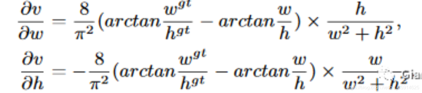
长宽在 [0,1]范围
计算的时候会变得很小。而在回归问题中回归很大的值是很难的,会导致梯度爆炸,因此在 
实现时将替换成1。
keras代码(没有替换为1,并且a求了梯度):
def box_ciou(b1, b2): """ 输入为: ---------- b1: tensor, shape=(batch, feat_w, feat_h, anchor_num, 4), xywh b2: tensor, shape=(batch, feat_w, feat_h, anchor_num, 4), xywh 返回为: ------- ciou: tensor, shape=(batch, feat_w, feat_h, anchor_num, 1) """ # 求出预测框左上角右下角 b1_xy = b1[..., :2] b1_wh = b1[..., 2:4] b1_wh_half = b1_wh/2. b1_mins = b1_xy - b1_wh_half b1_maxes = b1_xy + b1_wh_half # 求出真实框左上角右下角 b2_xy = b2[..., :2] b2_wh = b2[..., 2:4] b2_wh_half = b2_wh/2. b2_mins = b2_xy - b2_wh_half b2_maxes = b2_xy + b2_wh_half # 求真实框和预测框所有的iou intersect_mins = K.maximum(b1_mins, b2_mins) intersect_maxes = K.minimum(b1_maxes, b2_maxes) intersect_wh = K.maximum(intersect_maxes - intersect_mins, 0.) intersect_area = intersect_wh[..., 0] * intersect_wh[..., 1] b1_area = b1_wh[..., 0] * b1_wh[..., 1] b2_area = b2_wh[..., 0] * b2_wh[..., 1] union_area = b1_area + b2_area - intersect_area iou = intersect_area / (union_area + K.epsilon()) # 计算中心的差距 center_distance = K.sum(K.square(b1_xy - b2_xy), axis=-1) # 找到包裹两个框的最小框的左上角和右下角 enclose_mins = K.minimum(b1_mins, b2_mins) enclose_maxes = K.maximum(b1_maxes, b2_maxes) enclose_wh = K.maximum(enclose_maxes - enclose_mins, 0.0) # 计算对角线距离 enclose_diagonal = K.sum(K.square(enclose_wh), axis=-1) # calculate ciou, add epsilon in denominator to avoid dividing by 0 ciou = iou - 1.0 * (center_distance) / (enclose_diagonal + K.epsilon()) # calculate param v and alpha to extend to CIoU v = 4*K.square(tf.math.atan2(b1_wh[..., 0], b1_wh[..., 1]) - tf.math.atan2(b2_wh[..., 0], b2_wh[..., 1])) / (math.pi * math.pi) alpha = v / (1.0 - iou + v) ciou = ciou - alpha * v ciou = K.expand_dims(ciou, -1) return ciou
- 1
- 2
- 3
- 4
- 5
- 6
- 7
- 8
- 9
- 10
- 11
- 12
- 13
- 14
- 15
- 16
- 17
- 18
- 19
- 20
- 21
- 22
- 23
- 24
- 25
- 26
- 27
- 28
- 29
- 30
- 31
- 32
- 33
- 34
- 35
- 36
- 37
- 38
- 39
- 40
- 41
- 42
- 43
- 44
- 45
- 46
- 47
- 48
- 49
- 50
- 51
- 52
pytorch:
def bbox_overlaps_ciou(bboxes1, bboxes2): rows = bboxes1.shape[0] cols = bboxes2.shape[0] cious = torch.zeros((rows, cols)) if rows * cols == 0: return cious exchange = False if bboxes1.shape[0] > bboxes2.shape[0]: bboxes1, bboxes2 = bboxes2, bboxes1 cious = torch.zeros((cols, rows)) exchange = True w1 = bboxes1[:, 2] - bboxes1[:, 0] h1 = bboxes1[:, 3] - bboxes1[:, 1] w2 = bboxes2[:, 2] - bboxes2[:, 0] h2 = bboxes2[:, 3] - bboxes2[:, 1] area1 = w1 * h1 area2 = w2 * h2 center_x1 = (bboxes1[:, 2] + bboxes1[:, 0]) / 2 center_y1 = (bboxes1[:, 3] + bboxes1[:, 1]) / 2 center_x2 = (bboxes2[:, 2] + bboxes2[:, 0]) / 2 center_y2 = (bboxes2[:, 3] + bboxes2[:, 1]) / 2 inter_max_xy = torch.min(bboxes1[:, 2:],bboxes2[:, 2:]) inter_min_xy = torch.max(bboxes1[:, :2],bboxes2[:, :2]) out_max_xy = torch.max(bboxes1[:, 2:],bboxes2[:, 2:]) out_min_xy = torch.min(bboxes1[:, :2],bboxes2[:, :2]) inter = torch.clamp((inter_max_xy - inter_min_xy), min=0) inter_area = inter[:, 0] * inter[:, 1] inter_diag = (center_x2 - center_x1)**2 + (center_y2 - center_y1)**2 outer = torch.clamp((out_max_xy - out_min_xy), min=0) outer_diag = (outer[:, 0] ** 2) + (outer[:, 1] ** 2) union = area1+area2-inter_area u = (inter_diag) / outer_diag iou = inter_area / union with torch.no_grad(): arctan = torch.atan(w2 / h2) - torch.atan(w1 / h1) v = (4 / (math.pi ** 2)) * torch.pow((torch.atan(w2 / h2) - torch.atan(w1 / h1)), 2) S = 1 - iou alpha = v / (S + v) w_temp = 2 * w1 ar = (8 / (math.pi ** 2)) * arctan * ((w1 - w_temp) * h1) cious = iou - (u + alpha * ar) cious = torch.clamp(cious,min=-1.0,max = 1.0) if exchange: cious = cious.T return cious
- 1
- 2
- 3
- 4
- 5
- 6
- 7
- 8
- 9
- 10
- 11
- 12
- 13
- 14
- 15
- 16
- 17
- 18
- 19
- 20
- 21
- 22
- 23
- 24
- 25
- 26
- 27
- 28
- 29
- 30
- 31
- 32
- 33
- 34
- 35
- 36
- 37
- 38
- 39
- 40
- 41
- 42
- 43
- 44
- 45
- 46
- 47
- 48
- 49
- 50
文章来源: blog.csdn.net,作者:快了的程序猿小可哥,版权归原作者所有,如需转载,请联系作者。
原文链接:blog.csdn.net/qq_35914625/article/details/108528789

- 点赞
- 收藏
- 关注作者
评论(0)